Chapter 4 Model Checking in the Cox Regression Model

library(survival)
library(tidyverse)
library(flexsurv)
library(rms)
library(skimr)
library(stdReg)
library(survminer)

Survival_of_multiple_myeloma_patients <- read.table("./data/Survival of multiple myeloma patients.dat",
                                                    header=T)
d_1_3 <- Survival_of_multiple_myeloma_patients
d_1_3$sexf <- factor(d_1_3$sex)
d_1_3$proteinf <- factor(d_1_3$protein)
head(d_1_3)

##   patient time status age sex bun ca   hb pcells protein sexf proteinf
## 1       1   13      1  66   1  25 10 14.6     18       1    1        1
## 2       2   52      0  66   1  13 11 12.0    100       0    1        0
## 3       3    6      1  53   2  15 13 11.4     33       1    2        1
## 4       4   40      1  69   1  10 10 10.2     30       1    1        1
## 5       5   10      1  65   1  20 10 13.2     66       0    1        0
## 6       6    7      0  57   2  12  8  9.9     45       0    2        0

4.1 Einfalt Kaplan Meier

m1 <- survfit(Surv(time, status) ~ 1, data = d_1_3)

plot(m1)

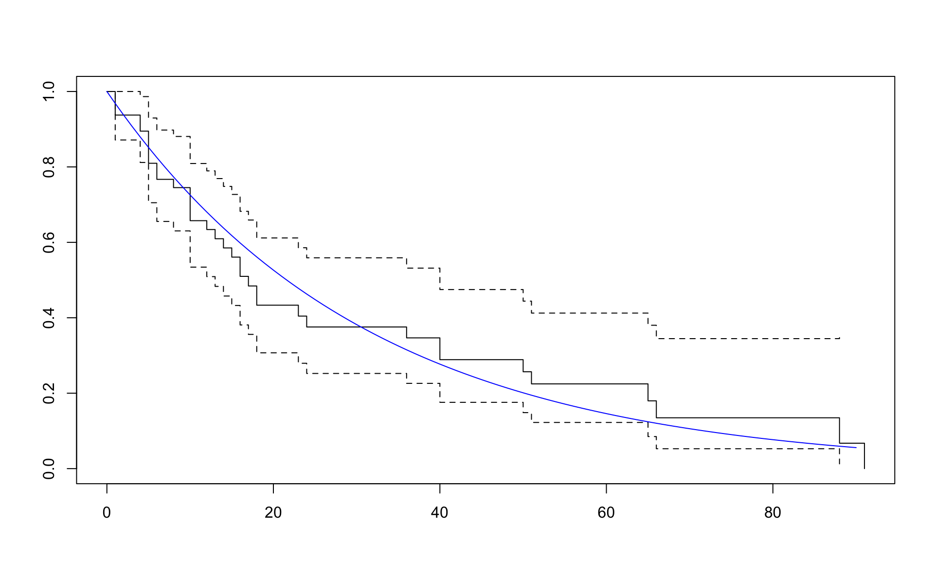
total_time <- sum(d_1_3$time)
num_events <- sum(d_1_3$status)
lambda <- num_events / total_time
lambda

## [1] 0.03208556

Tími á milli atburða er 1 / lambda

1 / lambda

## [1] 31.16667

4.2 Veldislifunarfallið

s <- function(t) exp(-lambda * t)
s(20)

## [1] 0.5263909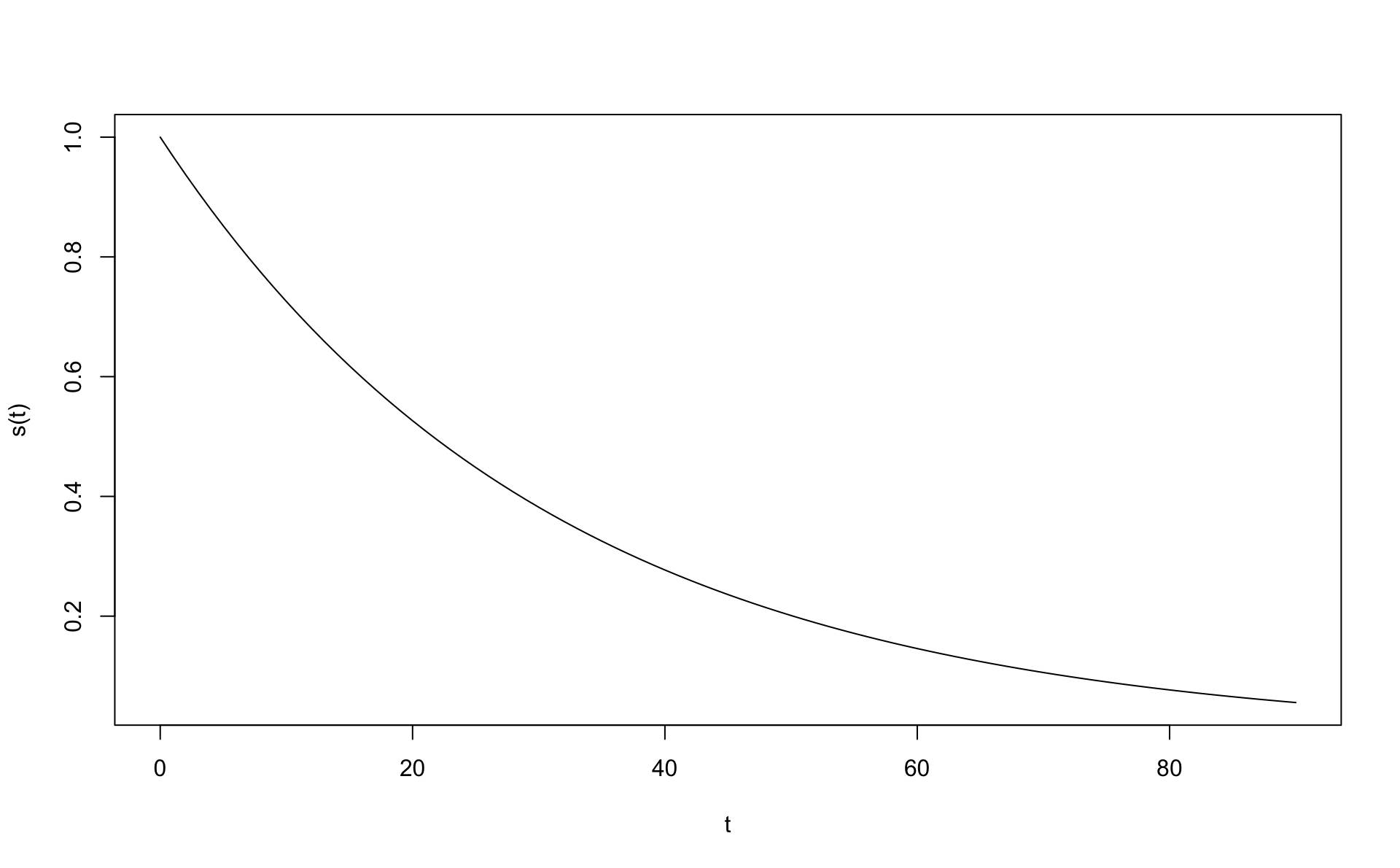

t <- seq(0, 90)
plot(t, s(t), type = "l")

plot(m1)
lines(x = t, y = s(t), col = "blue")

\[ S(t) = e^{-\lambda t} \]

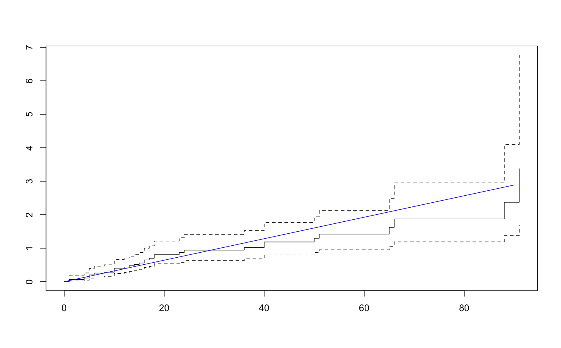
\[ H(t) = -\log S(t) = -\log (e^{-\lambda t}) = -(-\lambda t) = \lambda t \]

\[ H(t) = \int_0^t h(t)dt = \sum_{i=1}^n h(t)(t_{i + 1} - t_i) \]

plot(m1, fun = "cumhaz")
lines(t, lambda * t, col = "blue")

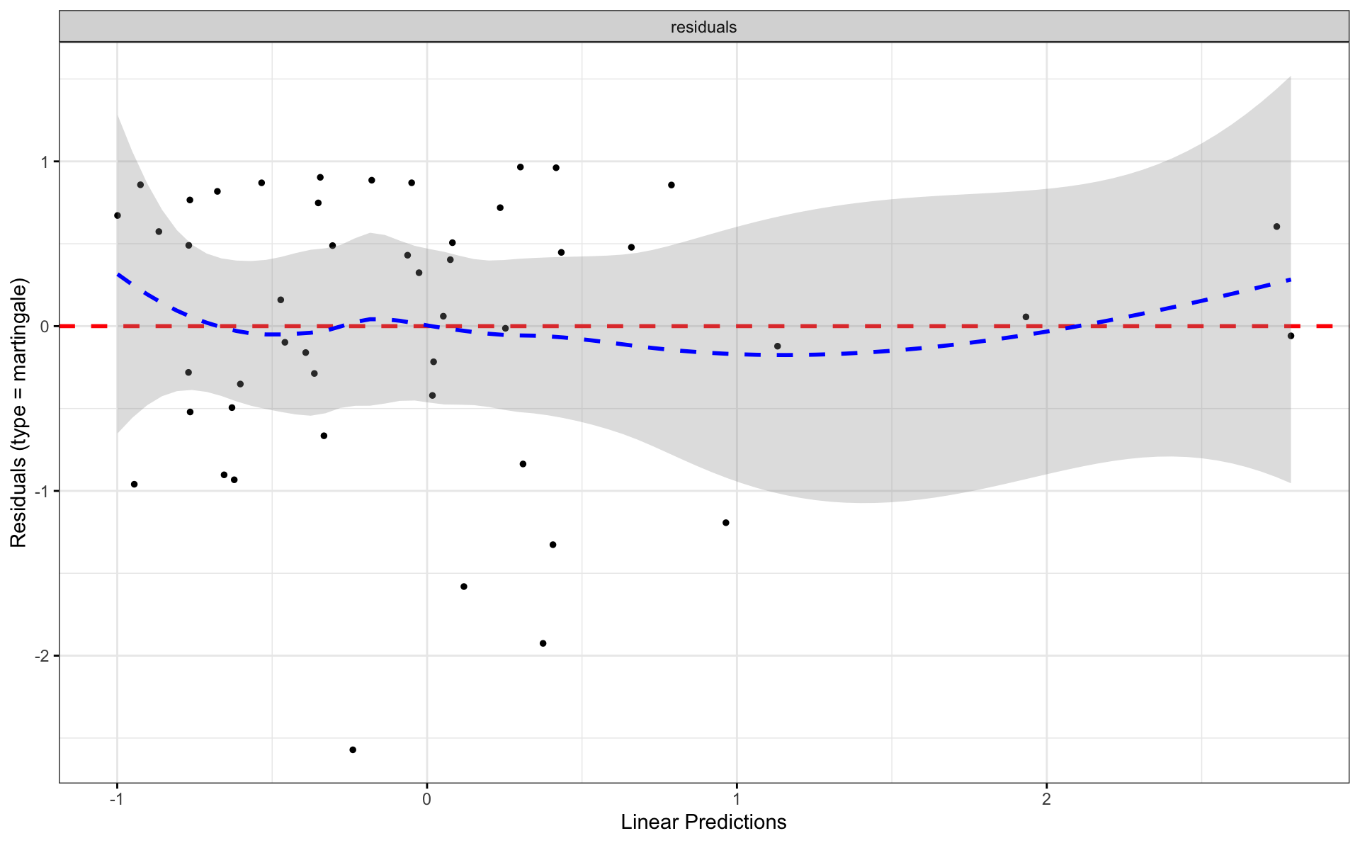
4.3 Leifar í Cox

head(d_1_3)

##   patient time status age sex bun ca   hb pcells protein sexf proteinf
## 1       1   13      1  66   1  25 10 14.6     18       1    1        1
## 2       2   52      0  66   1  13 11 12.0    100       0    1        0
## 3       3    6      1  53   2  15 13 11.4     33       1    2        1
## 4       4   40      1  69   1  10 10 10.2     30       1    1        1
## 5       5   10      1  65   1  20 10 13.2     66       0    1        0
## 6       6    7      0  57   2  12  8  9.9     45       0    2        0

m_4_5 <- coxph(Surv(time, status) ~ hb + bun, data = d_1_3)
m_4_5

## Call:
## coxph(formula = Surv(time, status) ~ hb + bun, data = d_1_3)
## 
##          coef exp(coef)  se(coef)      z        p
## hb  -0.134952  0.873758  0.061956 -2.178 0.029391
## bun  0.020043  1.020245  0.005816  3.446 0.000569
## 
## Likelihood ratio test=13.98  on 2 df, p=0.0009213
## n= 48, number of events= 36

Cox-Snell residuals eiga að hegða sér eins og lifunargögn úr veldisdreifingu með \(\lambda = 1\).

resid_martingale <- residuals(m_4_5, type = "martingale")
d_1_3$coxsnell <- d_1_3$status - resid_martingale

m_coxsnell <- survfit(Surv(coxsnell, status) ~ 1, data = d_1_3)

total_coxsnell <- sum(d_1_3$coxsnell)
lambda_coxsnell <- num_events / total_coxsnell
lambda_coxsnell

## [1] 1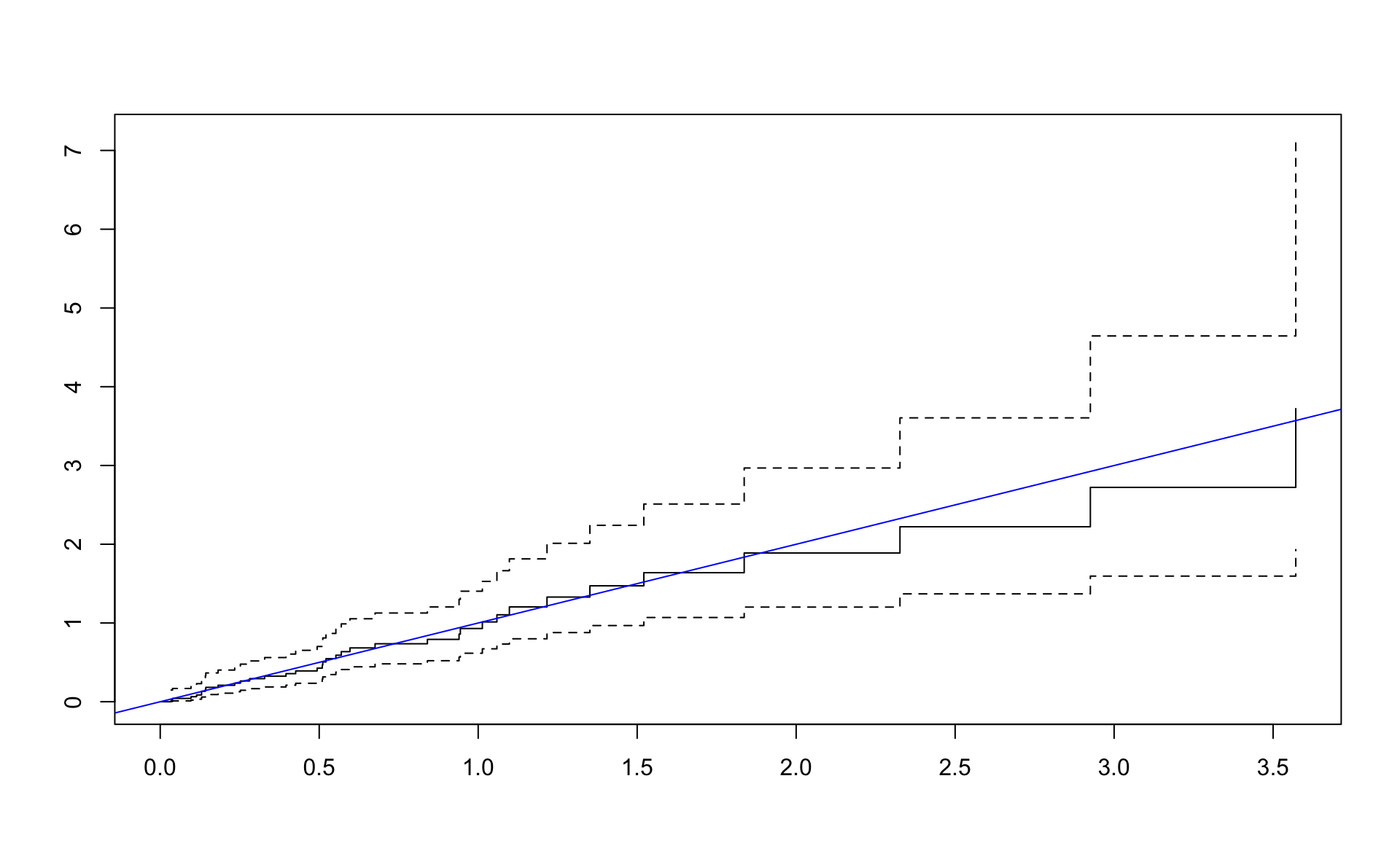

plot(m_coxsnell, fun = "cumhaz")
abline(a = 0, b = 1, col = "blue")

4.4 Survminer

ggcoxdiagnostics(m_4_5)

ggcoxfunctional(m_4_5)

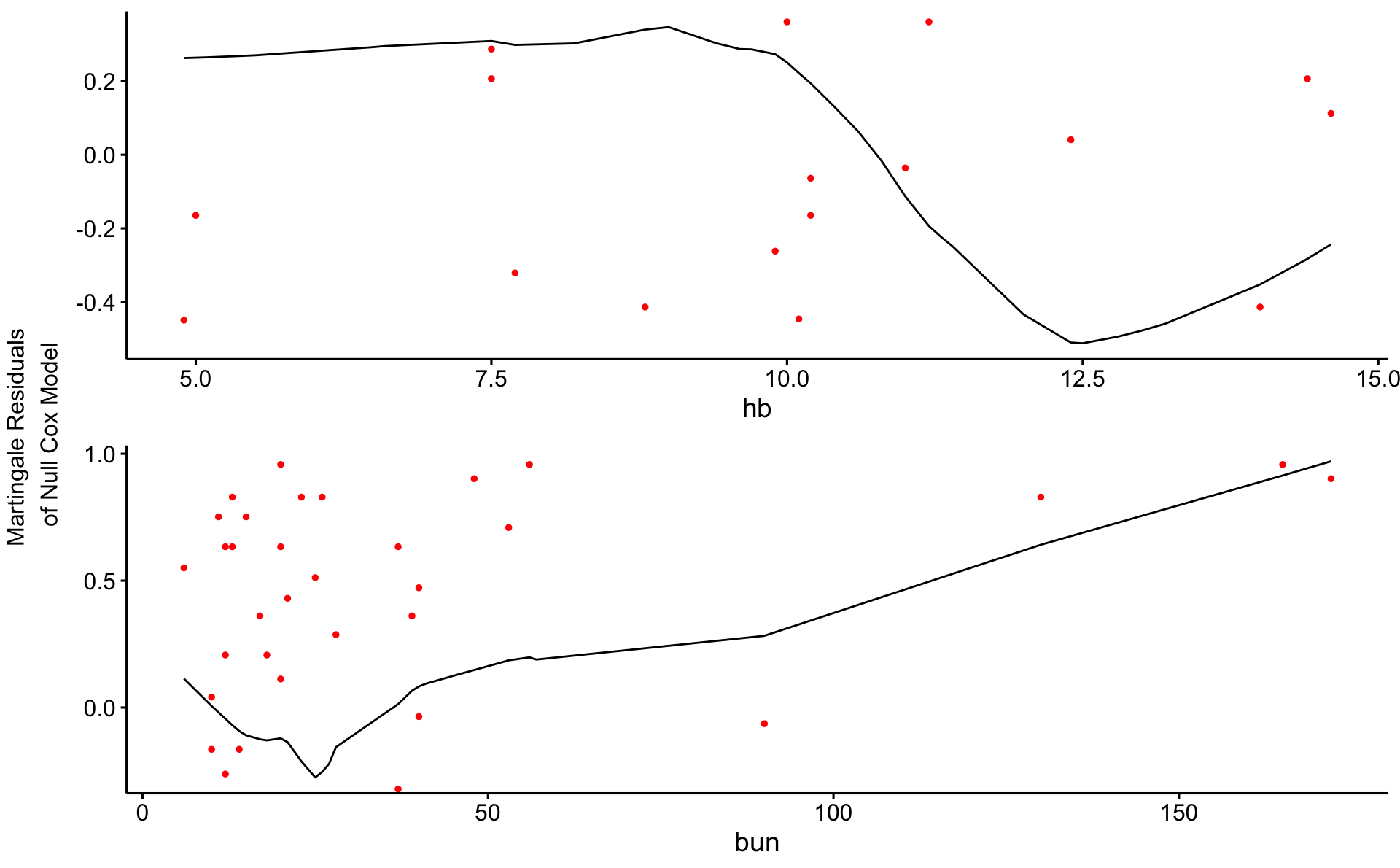
m_null <- coxph(Surv(time, status) ~ 1, data = d_1_3)
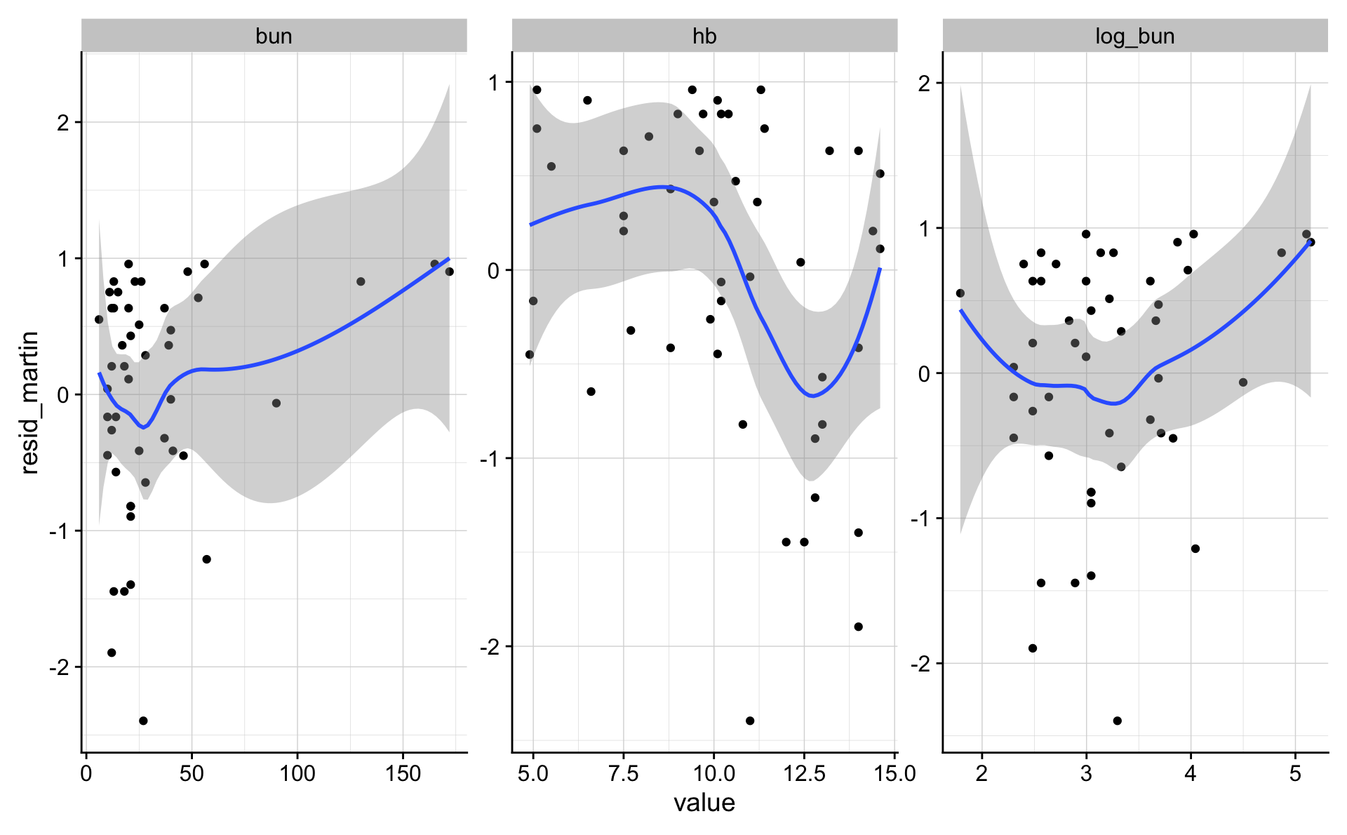
resid_martin <- residuals(m_null, type = "martingale")
d_1_3$resid_martin <- resid_martin

ggplot(data = d_1_3, aes(bun, resid_martin)) +
  geom_point() +
  geom_smooth(method = "loess") +
  scale_x_log10()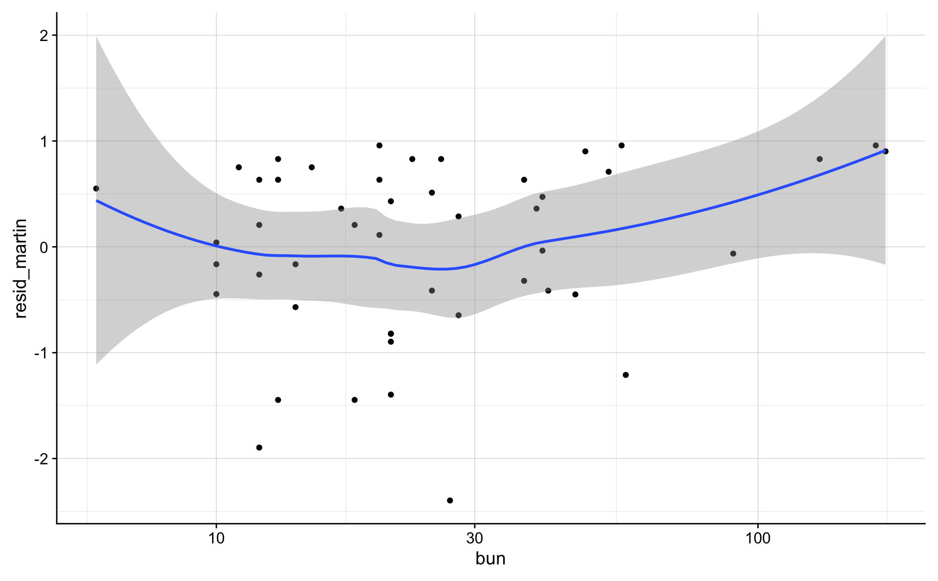

d_1_3 %>% 
  mutate(log_bun = log(bun)) %>% 
  gather(variable, value, log_bun, bun, hb) %>% 
  ggplot(aes(value, resid_martin)) +
  geom_point() +
  geom_smooth() +
  facet_wrap("variable", scales = "free")

4.4.1 Deviance residuals

ggcoxdiagnostics(m_4_5, type = "deviance")

4.4.2 dfbeta

ggcoxdiagnostics(m_4_5, type = "dfbeta")