It was the best of tails, it was the worst of tails: The T-Copula

library(tidyverse)
library(cmdstanr)
library(bayesplot)
library(patchwork)
library(gt)
theme_set(bggjphd::theme_bggj())

This post continues our series on copulas in Stan by introducing the t-copula and comparing it with the Gaussian copula we covered previously. We’ll focus particularly on how the t-copula’s tail dependence makes it more suitable for modeling extreme events.

Other posts in this series:

1. Introduction to Copulas in Stan
2. A Gentle Introduction: The Gaussian Copula

Note

This post assumes you’re familiar with the basics of copulas covered in the previous posts. If you’re new to copulas, I recommend starting with the introduction post.

Motivation: The Need for Tail Dependence

Before diving into the mathematical details, let’s understand why we need the t-copula in the first place. Consider the following scenarios:

1. Stock Market Crashes: During market crashes, stocks tend to fall together. The Gaussian copula can underestimate the probability of these joint extreme events.
2. Credit Default Modeling: The 2008 financial crisis highlighted the limitations of Gaussian copulas in modeling joint defaults. When one entity defaults, others are more likely to default as well - a phenomenon not well-captured by the Gaussian copula.
3. Natural Disasters: Extreme weather events often exhibit strong dependencies - when one measurement (temperature, rainfall, wind speed) reaches an extreme value, others are more likely to be extreme as well.

The t-copula addresses these limitations while maintaining many of the nice properties of the Gaussian copula.

In this post I might use Student-t and t exchangeably

A Quick Refresher on the Student-t Distribution

The Student-t distribution with \(\nu\) degrees of freedom can be viewed as arising from a normally distributed variable whose variability is adjusted by a random scaling factor derived from a chi-square distribution.

Formally, if we let \(Z \sim \mathcal{N}(0,1)\) and \(V \sim \chi^2_\nu\) be independent, then the t-distributed variable \(T\) can be defined as:

\[ T = \frac{Z}{\sqrt{V/\nu}}. \]

Here, \(Z\) represents a standardized normal deviate, and \(V/\nu\) acts like a variance estimate. As \(\nu\) grows large, the t-distribution approaches the standard normal distribution, and for smaller \(\nu\), the distribution exhibits heavier tails, capturing extreme values more frequently.

The T-Copula: A Dependent Tail

What is the t-Copula?

The t-copula is derived from the multivariate t-distribution, just as the Gaussian copula comes from the multivariate normal. It has two key parameters:

1. A correlation matrix \(\Sigma\) (like the Gaussian copula)
2. Degrees of freedom \(\nu\) (unique to the t-copula)

The degrees of freedom parameter \(\nu\) controls the heaviness of the tails:

• Lower values \(\to\) heavier tails \(\to\) stronger tail dependence
• Higher values \(\to\) lighter tails \(\to\) approaches the Gaussian copula
• As \(\nu \to \infty\), the t-copula becomes the Gaussian copula

Building Intuition: The Random Scale Factor

One of the most intuitive ways to understand the t-copula is through its stochastic representation:

1. Start with correlated normal variables \(\mathbf{Z} \sim \mathcal{N}(\mathbf{0}, \Sigma)\)
2. Generate a random scale factor \(W \sim \chi^2_\nu\)
3. Multiply everything by \(\sqrt{\nu/W}\) to get \(\mathbf{X} = \sqrt{\nu/W} \cdot \mathbf{Z}\)

This shared scaling creates tail dependence:

• When \(W\) is small, all variables become large together
• The smaller \(\nu\) is, the more variable \(W\) becomes
• This creates more frequent joint extreme events than the Gaussian copula

Understanding Tail Dependence

Before we proceed further, let’s formally define tail dependence. For a bivariate copula C, the upper and lower tail dependence coefficients are defined as:

\[ \begin{aligned} \lambda_U &= \lim_{u \to 1} P(U_2 > F_2^{-1}(u) | U_1 > F_1^{-1}(u)) \\ &= \lim_{u \to 1} \frac{1-2u+C(u,u)}{1-u} \\ \lambda_L &= \lim_{u \to 0} P(U_2 \leq F_2^{-1}(u) | U_1 \leq F_1^{-1}(u)) \\ &= \lim_{u \to 0} \frac{C(u,u)}{u} \end{aligned} \]

Intuitively, \(\lambda_U\) measures the probability that one variable is extremely large given that another is extremely large, while \(\lambda_L\) measures the probability that one variable is extremely small given that another is extremely small.

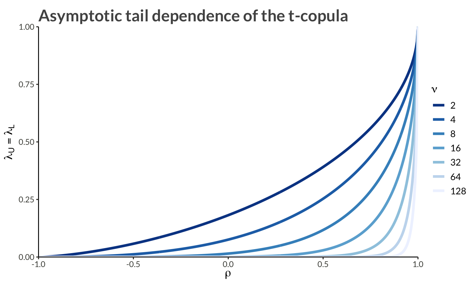
Due to radial symmetry, the t-copula has identical lower- and upper-tail dependence, given by:

\[ \lambda_U = \lambda_L = 2t_{\nu+1}\left(-\sqrt{\frac{(\nu + 1)(1-\rho)}{1+\rho}}\right) \]

where:

• \(t_{\nu+1}\) is the cumulative distribution function of a univariate t-distribution with \(\nu+1\) degrees of freedom
• \(\rho\) is the correlation parameter
• \(\nu\) is the degrees of freedom parameter

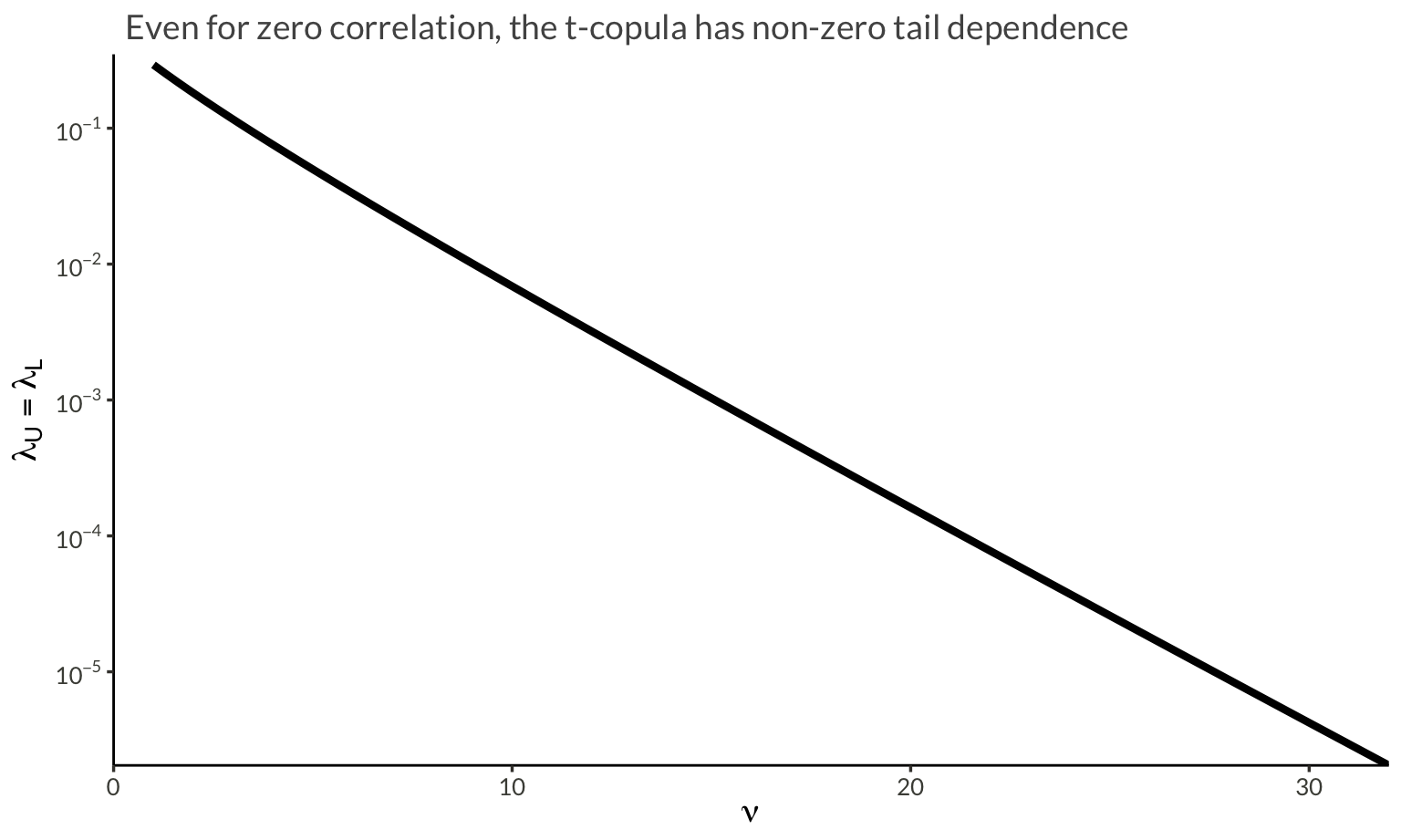
Some key properties of this tail dependence:

1. It is decreasing in \(\nu\) for fixed \(\rho\) (more degrees of freedom \(\to\) less tail dependence)
2. It is increasing in \(\rho\) for fixed \(\nu\) (stronger correlation \(\to\) stronger tail dependence)
3. As \(\nu \to \infty\), \(\lambda_U = \lambda_L \to 0\) for \(|\rho| < 1\), recovering the Gaussian case
4. For \(\rho = 1\), we have \(\lambda_U = \lambda_L = 1\) regardless of \(\nu\)
5. Even for \(\rho = 0\), we have non-zero tail dependence for finite \(\nu\).

t_tail_dependence <- function(rho, nu) {
  2 * pt(-sqrt((nu + 1) * (1 - rho) / (1 + rho)), nu + 1)
}

crossing(
  nu = c(2, 4, 8, 16, 32, 64, 128),
  rho = seq(-1, 1, length.out = 400)
) |>
  mutate(
    lambda = t_tail_dependence(rho, nu)
  ) |>
  ggplot(aes(rho, lambda, color = as.factor(nu))) +
  geom_line(
    linewidth = 1.5
  ) +
  scale_x_continuous(
    expand = c(0, 0),
    limits = c(-1, 1)
  ) +
  scale_y_continuous(
    expand = c(0, 0),
    limits = c(0, 1)
  ) +
  scale_colour_brewer(
    palette = "Blues",
    direction = -1
  ) +
  labs(
    x = expression(rho),
    y = expression(lambda[U] == lambda[L]),
    color = expression(nu),
    title = "Asymptotic tail dependence of the t-copula"
  )
crossing(
  nu = seq(1, 32, length.out = 100),
  rho = 0
) |>
  mutate(
    lambda = t_tail_dependence(rho, nu)
  ) |>
  ggplot(aes(nu, lambda)) +
  geom_line(linewidth = 1.5) +
  scale_x_continuous(
    expand = c(0, 0),
    limits = c(0, 32)
  ) +
  scale_y_continuous(
    expand = c(0, 0),
    limits = c(NA, 0.35),
    trans = "log10",
    labels = scales::label_log()
  ) +
  labs(
    x = expression(nu),
    y = expression(lambda[U] == lambda[L]),
    subtitle = "Even for zero correlation, the t-copula has non-zero tail dependence"
  )

Mathematical Definition

Now that we have the intuition, let’s look at the formal definition. Let \(\mathbf X = (X_1, \dots, X_D)\) be a multivariate random variable with marginal distribution functions \(F_i\) and dependence according to the t-copula. Their joint distribution function and density can be written: \[ \begin{aligned} H(\mathbf{X}) &= t_{\nu,\Sigma}\left(t_\nu^{-1}(F_1(X_1)), \dots, t_\nu^{-1}(F_D(X_D))\right) \\ h(\mathbf{X}) &= c\left(F_1(X_1), \dots, F_D(X_D)\right)\prod_{i=1}^D f_i(X_i) \end{aligned} \]

where:

• \(H(\mathbf X)\) is the joint cumulative distribution function (CDF) of the collection of random variables \(\mathbf X\)
• \(h(\mathbf X)\) is the joint density corresponding to the CDF, \(H(\mathbf X)\)
• \(t_{\nu,\Sigma}\) is the CDF of the multivariate t-distribution with \(\nu\) degrees of freedom and correlation matrix \(\Sigma\)
• \(t_\nu^{-1}\) is the inverse CDF of the univariate t-distribution with \(\nu\) degrees of freedom
• \(F_i\) and \(f_i\) are the marginal CDFs and PDFs

The log-density of the t-copula can be written as: \[ \begin{aligned} \log c(\mathbf{u}|\nu,\Sigma) &= \log t_{\nu,\Sigma}(\mathbf{z}) - \sum_{i=1}^D \log t_\nu(z_i) \\ z_i &= t_\nu^{-1}(u_i) \end{aligned} \]

where \(t_{\nu,\Sigma}\) is the multivariate t density with correlation matrix \(\Sigma\) and \(t_\nu\) is the univariate t density.

Key Properties

Tail Dependence

Unlike the Gaussian copula, the t-copula exhibits tail dependence. The upper and lower tail dependence coefficients are:

\[ \lambda_U = \lambda_L = 2t_{\nu+1}\left(-\sqrt{\frac{(\nu + 1)(1-\rho)}{1+\rho}}\right) \]

This symmetry (\(\lambda_U = \lambda_L\)) means the t-copula treats both tails equally.

Limiting Cases

• As \(\nu \to \infty\): Converges to Gaussian copula
• As \(\nu \to 0\): Tail dependence increases¹
• \(\nu = 1\): Cauchy copula (strongest tail dependence)

¹ Lower values of \(\nu\) produce heavier tails and increase tail dependence. However, taking \(\nu\) extremely close to zero is more of a theoretical construct than a practical modeling choice. In most applications, \(\nu\) is chosen within a range that provides heavier tails than the Gaussian case, but not so extreme as to be unrealistic.

Concordance Measures

Like the Gaussian copula:

• Kendall’s \(\tau\): \(\tau = \frac{2}{\pi}\arcsin(\rho)\)
• Spearman’s \(\rho\): \(\rho_S = \frac{6}{\pi}\arcsin(\rho/2)\)

where \(\rho\) is the correlation coefficient.²

² Note that these concordance measures are identical to the Gaussian copula because multiplying by the scaling factor \(\sqrt{\nu/W}\) affects the magnitude of the variables but preserves their ranks. Since Kendall’s \(\tau\) and Spearman’s \(\rho\) only depend on the ranks of the data, not their actual values, they remain unchanged from the Gaussian case.

An Example

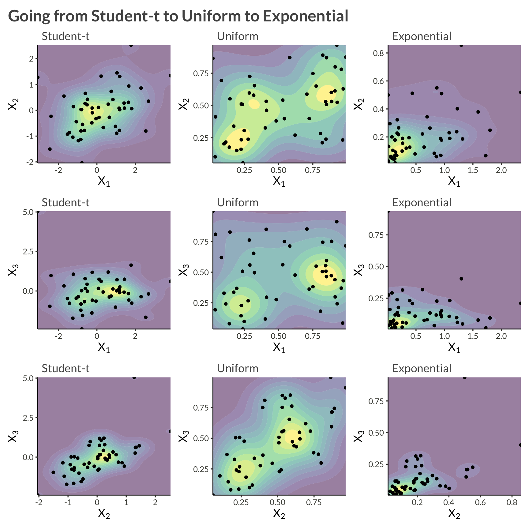
Let’s use the same example as in the previous post, except now with three variables, \(Y_1\) and \(Y_2\) and \(Y_3\). We will model each asset’s marginal distribution as exponential, and apply a multivariate t-copula to model their dependence. Alltogether this can be written \[ \log h(\mathbf{Y}) = \log t_{\nu, \Sigma}(z_1, z_2, z_3 \vert \Sigma) - \log t_\nu(z_1, z_2, z_3) + \sum_{i=1}^3 f_{\mathrm{Exp}}(Y_i \vert \lambda_i) \]

Sampling the Data

In words

To sample from this data-generating process we

1. Generate \(\mathbf{Z} \sim \mathcal{N}(\mathbf{0}, \mathbf{I}_D)\)
2. Generate \(W \sim \chi^2(\nu)\) independently
3. Apply correlation structure: \(\mathbf{Z}' = \mathbf{L}\mathbf{Z}\)
4. Scale variables: \(\mathbf{X} = \sqrt{\nu/W}\cdot\mathbf{Z}'\)
5. Transform to uniform: \(\mathbf{U} = t_\nu(\mathbf{X})\)
6. Transform to exponential: \(\mathbf{Y} = F^{-1}_{\text{Exp}}(\mathbf{U}|\boldsymbol{\lambda})\)

In code

n_obs <- 50
rho12 <- 0.8
rho13 <- 0.1
rho23 <- 0.4
lambda1 <- 2
lambda2 <- 4
lambda3 <- 6
df <- 4
sigma <- matrix(
  c(
    1, rho12, rho13,
    rho12, 1, rho23,
    rho13, rho23, 1
  ),
  nrow = 3
)
L <- chol(sigma)

set.seed(1)
W <- rchisq(n_obs, df = df)
Z <- matrix(rnorm(n = n_obs * 3), nrow = 3)
Z <- sqrt(df / W) * t(L %*% Z)

d <- tibble(
  z1 = Z[, 1],
  z2 = Z[, 2],
  z3 = Z[, 3],
  time = seq_len(n_obs)
)  |> 
  pivot_longer(
    c(-time), 
    names_to = "variable", 
    names_transform = parse_number,
    values_to = "z"
  ) |> 
  inner_join(
    tibble(
      variable = c(1, 2, 3),
      lambda = c(lambda1, lambda2, lambda3)
    )
  ) |> 
  mutate(
    u = pt(z, df = df),
    y = qexp(u, rate = lambda)
  )

d |>
  select(-lambda) |>
  pivot_longer(c(z, u, y)) |>
  pivot_wider(names_from = variable, names_prefix = "v") |>
  mutate(
    name = fct_relevel(name, "z", "u") |>
      fct_recode(
        "Student-t" = "z",
        "Uniform" = "u",
        "Exponential" = "y"
      )
  ) |>
  group_by(n2 = name) |>
  group_map(
    \(data, ...) {
      # X2 vs X1
      p12 <- data |>
        ggplot(aes(v1, v2)) +
        geom_density_2d_filled(alpha = 0.5) +
        geom_point(size = 1.4) +
        scale_x_continuous(
          expand = c(0, 0)
        ) +
        scale_y_continuous(
          expand = c(0, 0)
        ) +
        theme(legend.position = "none") +
        labs(
          subtitle = unique(data$name),
          x = expression(X[1]),
          y = expression(X[2])
        )

      # X3 vs X1
      p13 <- data |>
        ggplot(aes(v1, v3)) +
        geom_density_2d_filled(alpha = 0.5) +
        geom_point(size = 1.4) +
        scale_x_continuous(
          expand = c(0, 0)
        ) +
        scale_y_continuous(
          expand = c(0, 0)
        ) +
        theme(legend.position = "none") +
        labs(
          subtitle = unique(data$name),
          x = expression(X[1]),
          y = expression(X[3])
        )

      # X3 vs X2
      p23 <- data |>
        ggplot(aes(v2, v3)) +
        geom_density_2d_filled(alpha = 0.5) +
        geom_point(size = 1.4) +
        scale_x_continuous(
          expand = c(0, 0)
        ) +
        scale_y_continuous(
          expand = c(0, 0)
        ) +
        theme(legend.position = "none") +
        labs(
          subtitle = unique(data$name),
          x = expression(X[2]),
          y = expression(X[3])
        )

      wrap_plots(p12, p13, p23, nrow = 3)
    }
  ) |>
  wrap_plots(
    ncol = 3,
    widths = c(1, 1,1 )
  ) +
  plot_annotation(
    title = "Going from Student-t to Uniform to Exponential"
  )

Stan Model

The Stan implementation has three main components:

Student-t Copula Log-Density

Similar to the Gaussian copula, we need to implement the t-copula log density:

real t_copula_lpdf(vector u, matrix L, real nu) {
  int D = num_elements(u);
  vector[D] x;
  real logp;

  // Transform U to X via the inverse t CDF
  for (d in 1:D) {
    x[d] = student_t_icdf(u[d], nu);
  }

  // Multivariate t density minus sum of univariate t densities
  logp = multi_student_t_cholesky_lpdf(x | nu, rep_vector(0, D), L);
  for (d in 1:D) {
    logp -= student_t_lpdf(x[d] | nu, 0, 1);
  }

  return logp;
}

The key differences from the Gaussian copula are:

1. We use the t-distribution’s quantile function instead of the normal quantile function
2. We use the multivariate t-distribution instead of the multivariate normal
3. We have an additional parameter nu for the degrees of freedom

Student-t Quantile Function:

Unlike the Gaussian copula where we could use Stan’s built-in inv_Phi(), we need to implement the t-distribution’s quantile function ourselves. The implementation in the Stan model follows numerical approximations for different ranges of the input values to ensure stability and accuracy.

The function is too long to paste here, but it is based on Sean Pinkey’s implementation from the Stan forums

Model Specification

The model follows a similar structure to the Gaussian copula but with the addition of the degrees of freedom parameter:

parameters {
  vector<lower=0>[D] lambda;
  cholesky_factor_corr[D] L;
  real<lower=1> nu;   // degrees of freedom for the t-copula
}

model {
  matrix[N, D] U;
  for (i in 1:N) {
    // Transform data to uniforms using exponential CDF
    for (j in 1:D) {
      target += exponential_lpdf(Y[i, j] | lambda[j]);
      U[i, j] = exponential_cdf(Y[i, j] | lambda[j]);
    }
    // Add the t-copula contribution
    target += t_copula_lpdf(to_vector(U[i, ]) | L, nu);
  }

  // Priors
  target += lkj_corr_cholesky_lpdf(L | 1.0);
  target += exponential_lpdf(nu | 1);
  target += exponential_lpdf(lambda | 1);
}

Generated Quantities

For posterior predictive checks, we need to:

1. Generate samples from the multivariate t-distribution
2. Transform them to uniform variables using the t CDF
3. Transform to exponential variables using the exponential quantile function

generated quantities {
  corr_matrix[D] Sigma = multiply_lower_tri_self_transpose(L);
  matrix[N, D] yrep;

  {
    matrix[N, D] U_rep;
    matrix[N, D] Z_rep;

    for (i in 1:N) {
      Z_rep[i] = (multi_student_t_cholesky_rng(nu, rep_vector(0, D), L))';
      for (j in 1:D) {
        U_rep[i, j] = student_t_cdf(Z_rep[i, j] | nu, 0, 1);
        yrep[i, j] = exponential_icdf(U_rep[i, j], lambda[j]);
      }
    }
  }
}

The main differences from the Gaussian copula’s generated quantities block are:

1. We use multi_student_t_cholesky_rng() instead of multi_normal_cholesky_rng()
2. We use student_t_cdf() instead of Phi()
3. The degrees of freedom parameter nu is passed to both functions
4. This implementation allows us to model tail dependence that the Gaussian copula cannot capture, while maintaining the same marginal distributions.

Sampling from the posterior

Prepare the data and sample from the model.

Y <- d |>
  select(time, variable, y) |> 
  pivot_wider(names_from = variable, values_from = y) |> 
  select(-time) |> 
  as.matrix()

stan_data <- list(
  Y = Y,
  N = nrow(Y),
  D = ncol(Y)
)

example1 <- cmdstan_model(here::here("posts", "t-copula", "Stan", "t-copula.stan"))

result <- example1$sample(
  data = stan_data,
  chains = 4,
  seed = 1,
  parallel_chains = 4,
  show_messages = FALSE,
  show_exceptions = FALSE
)

result$summary(c("lambda", "Sigma[1,2]", "Sigma[1,3]", "Sigma[2,3]", "nu")) |> 
  gt() |> 
  fmt_number()

variable	mean	median	sd	mad	q5	q95	rhat	ess_bulk	ess_tail
lambda[1]	1.53	1.52	0.20	0.19	1.22	1.86	1.00	3,394.27	2,825.60
lambda[2]	3.57	3.55	0.50	0.51	2.79	4.45	1.00	2,607.47	2,528.29
lambda[3]	6.08	6.05	0.79	0.78	4.85	7.44	1.00	2,922.44	2,475.93
Sigma[1,2]	0.43	0.44	0.12	0.12	0.21	0.61	1.00	2,873.68	2,756.21
Sigma[1,3]	0.19	0.20	0.13	0.14	−0.04	0.41	1.00	2,875.84	2,802.58
Sigma[2,3]	0.74	0.75	0.08	0.07	0.60	0.84	1.00	3,029.44	2,799.22
nu	3.55	3.29	1.23	1.07	2.00	5.88	1.00	3,499.92	2,999.41

mcmc_trace(
  result$draws(), 
  pars = c("lambda[1]", "lambda[2]", "Sigma[1,2]", "nu")
  )

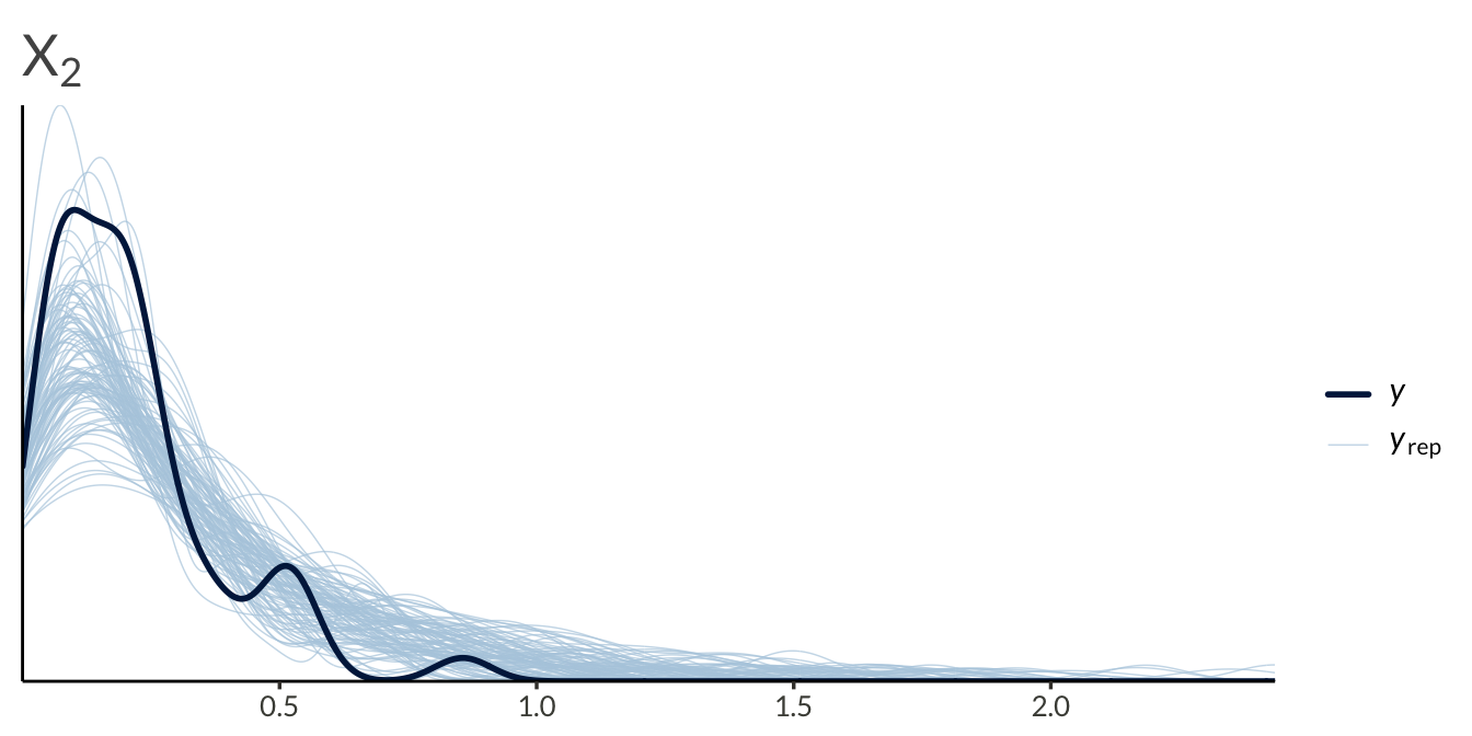
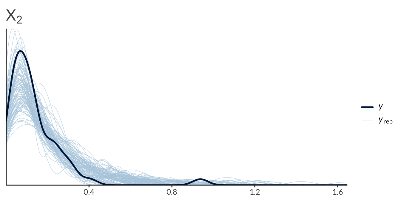
yrep <- result$draws("yrep", format = "matrix")
y <- as.numeric(Y)

ppc_dens_overlay(
  y = y[seq_len(n_obs)], 
  yrep = yrep[1:100, seq_len(n_obs)]
) + 
  ggtitle(expression(X[1]))
ppc_dens_overlay(
  y = y[n_obs + seq_len(n_obs)], 
  yrep = yrep[1:100, n_obs + seq_len(n_obs)]
) +
  ggtitle(expression(X[2]))
ppc_dens_overlay(
  y = y[2 * n_obs + seq_len(n_obs)], 
  yrep = yrep[1:100, 2 * n_obs + seq_len(n_obs)]
) +
  ggtitle(expression(X[2]))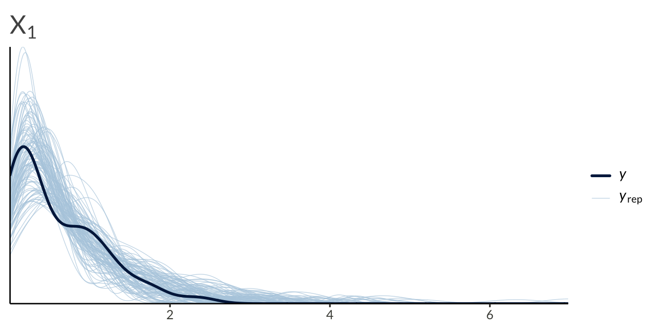

Some Facts About the t-Copula

1. Dependence Range and Structure:
   • Like the Gaussian copula, interpolates between independence (\(\rho=0\)) and perfect dependence (\(\rho=\pm1\))
   • Tail dependence controlled by degrees of freedom parameter \(\nu\)
   • Lower values of \(\nu\) produce stronger tail dependence
   • As \(\nu \to \infty\), converges to the Gaussian copula
   • As \(\nu \to 0\), tail dependence increases
2. Concordance Measures:
   • Identical to the Gaussian copula due to rank preservation:
     • Kendall’s \(\tau\): \(\tau = \frac{2}{\pi}\arcsin(\rho)\)
     • Spearman’s \(\rho_S\): \(\rho_S = \frac{6}{\pi}\arcsin(\rho/2)\)
   • This is because multiplying by the scaling factor \(\sqrt{\nu/W}\) affects magnitude but preserves ranks
3. Symmetries and Dependencies:
   • Radial Symmetry: Like the Gaussian copula, exhibits radial symmetry
   • Exchangeability: For bivariate case, invariant under permutation of arguments
   • Tail Dependence: Unlike Gaussian copula, has tail dependence:
     • Upper and lower tail dependence coefficients are equal: \(\lambda_U = \lambda_L = 2t_{\nu+1}\left(-\sqrt{\frac{(\nu + 1)(1-\rho)}{1+\rho}}\right)\)
     • Cannot model asymmetric tail dependence scenarios
     • Tail dependence persists even with zero correlation
4. Computational Considerations:
   • More complex to implement than Gaussian copula
   • Requires careful numerical handling of t quantile function
   • Parameter estimation more challenging due to additional \(\nu\) parameter
5. Practical Applications:
   • Well-suited for financial data where extreme co-movements are common
   • Better than Gaussian for modeling joint extreme events
   • Popular in risk management due to tail dependence properties
   • Useful when data shows symmetric heavy-tailed behavior
6. Limitations:
   • Cannot capture asymmetric tail dependence
   • Symmetric tail dependence may not match all applications

Looking ahead

While the t-copula addresses some limitations of the Gaussian copula through tail dependence, it still maintains symmetries that may not be appropriate for all applications. The next posts will be about Archimedean copulas, which can model:

• Asymmetric tail dependence
• Different dependence structures
• More flexible patterns of association