The Smooth Step

library(bggjphd)
library(tidyverse)
library(bayesplot)
library(posterior)
library(GGally)
library(scales)
library(cowplot)
library(kableExtra)
library(arrow)
theme_set(theme_bggj())

The latent parameters, \(\psi\), \(\tau\), \(\phi\), and \(\gamma\), are given intrinsic random walk spatial priors, for example

\[ \begin{aligned} \psi &\sim \mathcal N(\mathbf 0, \tau_\psi \cdot Q_u) \\ \sigma_\psi &= \frac{1}{\sqrt\tau_\psi} \\ \sigma_\psi &\sim \mathrm{Exp}(1) \end{aligned} \]

Here, \(Q_u\) is defined by

\[ Q_u = R \otimes I + I \otimes R, \]

where \(I\) is the identity matrix and

\[ R = \begin{bmatrix} 1 & -1 & & & & & \\ -1 & 2 & -1 & & & & \\ & -1 & 2 & -1 & & & \\ & & \ddots & \ddots & \ddots & & \\ & & &-1 &2 &-1 & \\ & & & & -1 & 1\\ \end{bmatrix}. \]

The results were obtained by running ms_smooth() in parrallel on four cores with four chains each run for 4000 samples. Half of those samples were designated as warm-up and so we have a total of 8000 samples from the posterior.

theta_results <- read_parquet("data/theta_results.parquet") |> 
  as_draws_df()

station_results <- read_parquet("data/station_results.parquet")

n_iter <- theta_results |> 
  as_tibble() |> 
  pull(.iteration) |> 
  max()

MCMC Diagnostics

Trace plots

theta_results |> 
  filter(.chain != 4) |> 
  filter(.iteration > 1) |>
  mcmc_trace()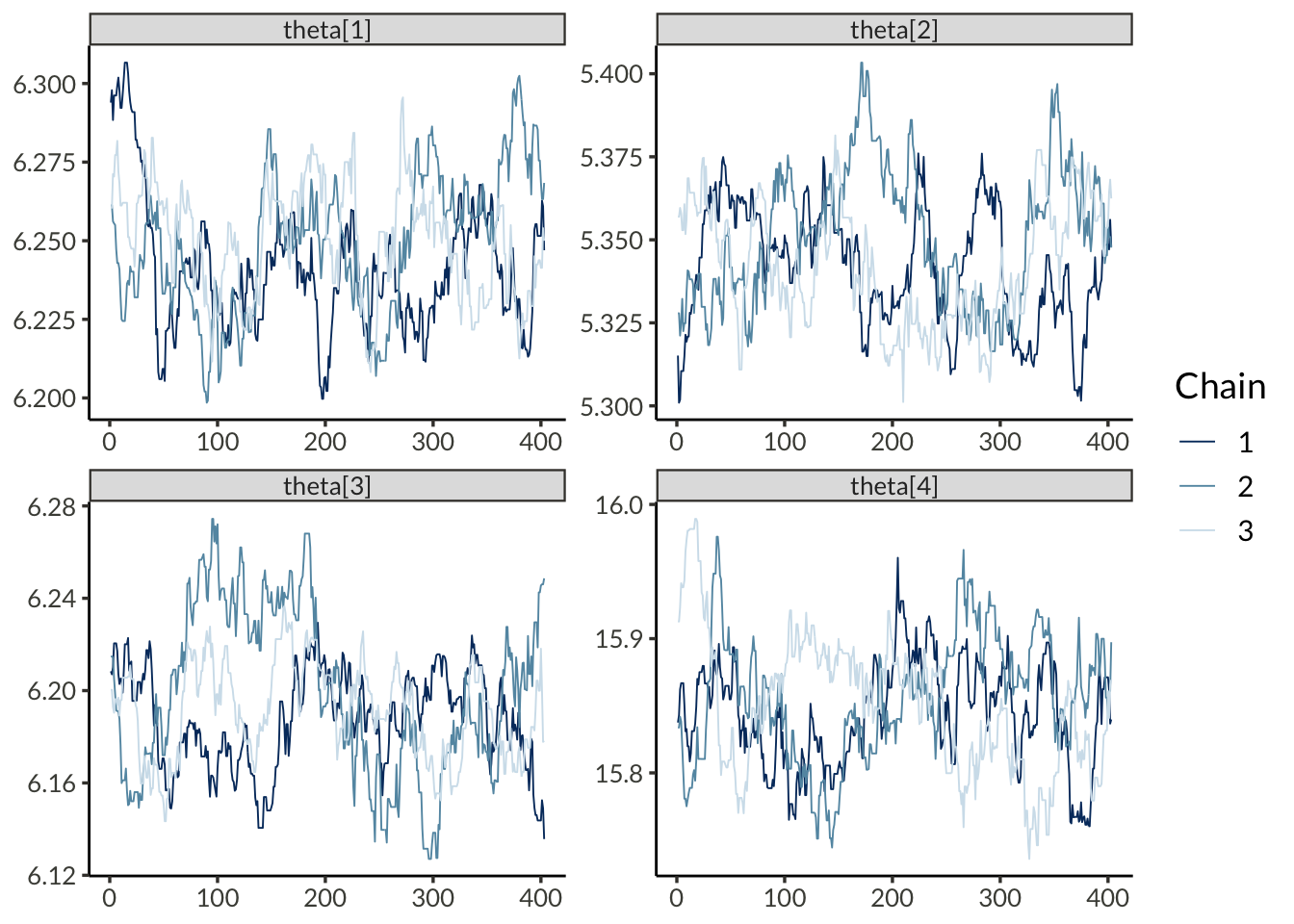

Autocorrelation functions

theta_results |> 
  filter(.iteration > 1) |> 
  mcmc_acf_bar()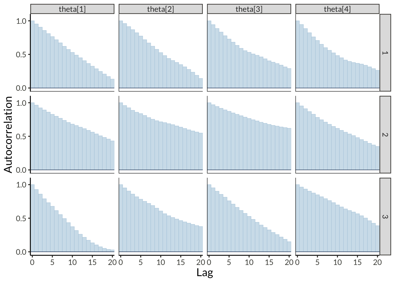

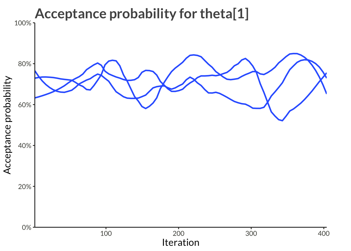
Acceptance probability

theta_results |> 
  subset_draws("theta[1]") |> 
  as_tibble() |> 
  rename(value = "theta[1]") |> 
  group_by(.chain) |> 
  mutate(accept = 1 * (value != lag(value))) |> 
  ungroup() |> 
  ggplot(aes(.iteration, accept, group = .chain)) +
  geom_smooth(method = "loess", span = 0.3, se = 0) +
  scale_x_continuous(
    expand = expansion()
  ) +
  scale_y_continuous(
    breaks = pretty_breaks(5),
    labels = label_percent(),
    expand = expansion()
  ) +
  theme(
    plot.margin = margin(t = 5, r = 35, b = 5, l = 5)
  ) +  
  coord_cartesian(ylim = c(0, 1)) +
  labs(
    x = "Iteration",
    y = "Acceptance probability",
    title = "Acceptance probability for theta[1]"
  )

Parameters

Hyperpriors

Log precision scale

theta_results |> 
  filter(.iteration > 1) |> 
  summarise_draws() |> 
  kable(digits = 3) |> 
  kable_styling(bootstrap_options = c("striped", "hover"))

variable	mean	median	sd	mad	q5	q95	rhat	ess_bulk	ess_tail
theta[1]	6.247	6.247	0.020	0.022	6.215	6.282	1.068	41.341	55.597
theta[2]	5.345	5.345	0.019	0.022	5.315	5.375	1.056	30.657	53.149
theta[3]	6.193	6.192	0.027	0.027	6.151	6.243	1.141	16.002	16.160
theta[4]	15.850	15.851	0.045	0.047	15.775	15.923	1.172	14.069	65.501

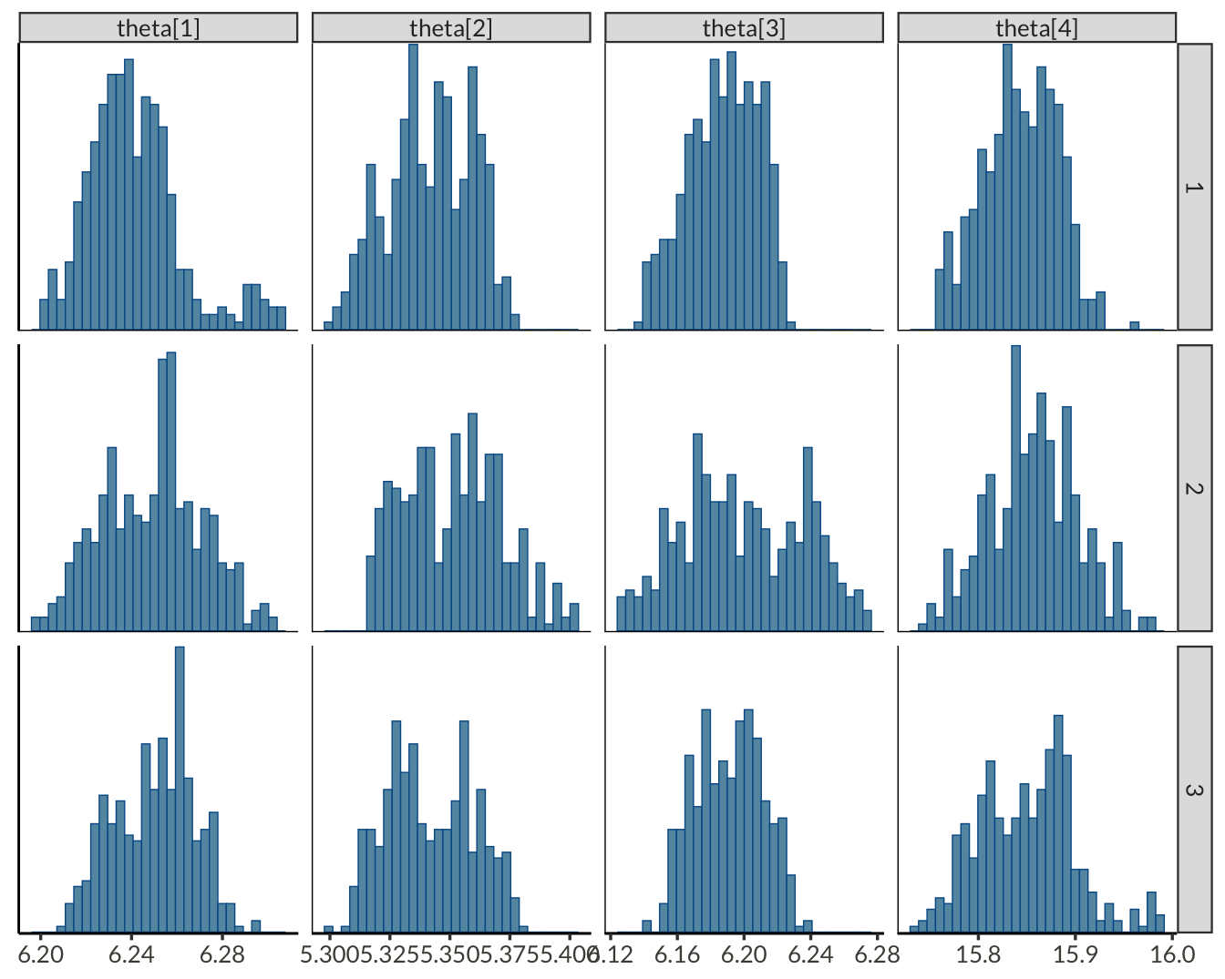
theta_results |> 
  filter(.iteration > 1) |> 
  mcmc_hist_by_chain(
  )

On standard deviation scale

theta_results |> 
  filter(.iteration > 1) |> 
  summarise_draws() |> 
  kable(digits = 3) |> 
  kable_styling(bootstrap_options = c("striped", "hover"))

variable	mean	median	sd	mad	q5	q95	rhat	ess_bulk	ess_tail
theta[1]	6.247	6.247	0.020	0.022	6.215	6.282	1.068	41.341	55.597
theta[2]	5.345	5.345	0.019	0.022	5.315	5.375	1.056	30.657	53.149
theta[3]	6.193	6.192	0.027	0.027	6.151	6.243	1.141	16.002	16.160
theta[4]	15.850	15.851	0.045	0.047	15.775	15.923	1.172	14.069	65.501

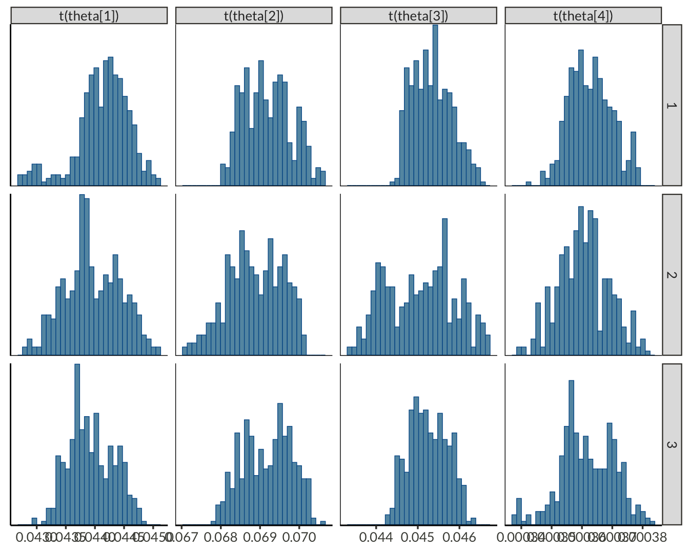
theta_results |> 
  filter(.iteration > 1) |> 
  mcmc_hist_by_chain(
    transformations = function(x) exp(-x/2)
  )

GEV Parameters

Comparing ML and MCMC estimates

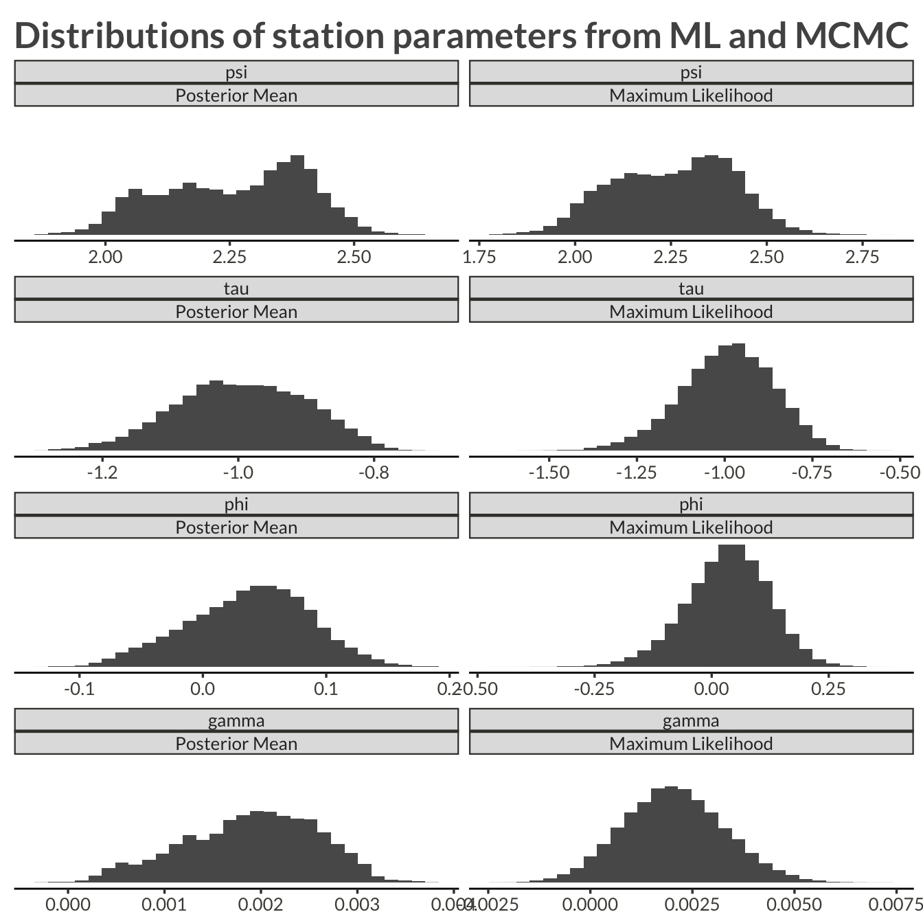
station_results |> 
  pivot_longer(c(ml_estimate, mcmc_mean)) |> 
  mutate(
    variable = fct_relevel(
      factor(variable),
      "psi", "tau", "phi", "gamma"
    ),
    name = fct_recode(
      factor(name),
      "Maximum Likelihood" = "ml_estimate",
      "Posterior Mean" = "mcmc_mean"
    )
  ) |> 
  ggplot(aes(value)) +
  geom_histogram() +
  facet_wrap(vars(variable, name), ncol = 2, scales = "free_x") +
  theme(
    axis.line.y = element_blank(),
    axis.text.y = element_blank(),
    axis.ticks.y = element_blank()
  ) +
  labs(
    x = NULL,
    y = NULL,
    title = "Distributions of station parameters from ML and MCMC"
  )

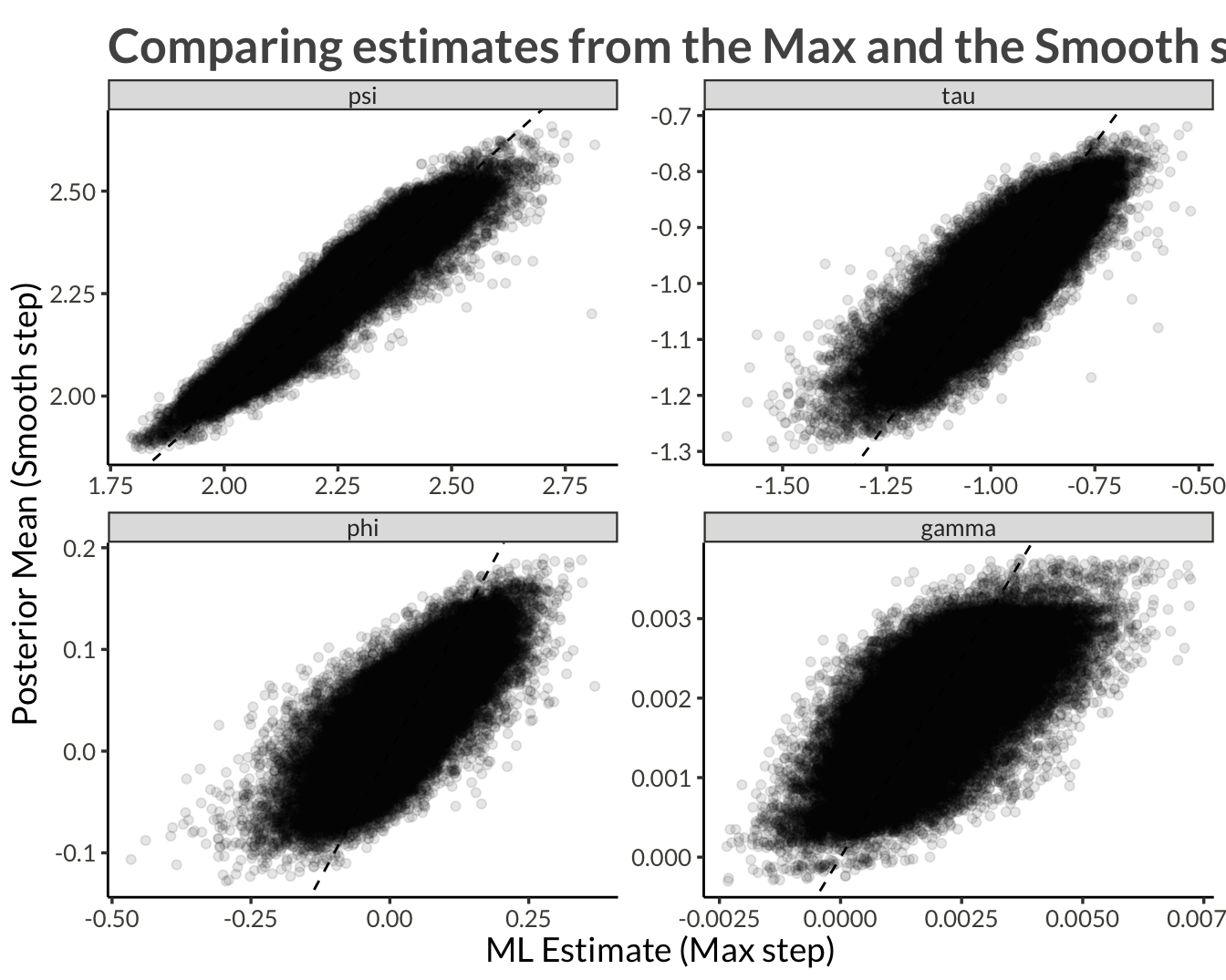
station_results |> 
  ggplot(aes(ml_estimate, mcmc_mean)) +
  geom_abline(intercept = 0, slope = 1, lty = 2) +
  geom_point(alpha = 0.1) +
  facet_wrap("variable", scales = "free") +
  labs(
    x = "ML Estimate (Max step)",
    y = "Posterior Mean (Smooth step)",
    title = "Comparing estimates from the Max and the Smooth steps"
  )

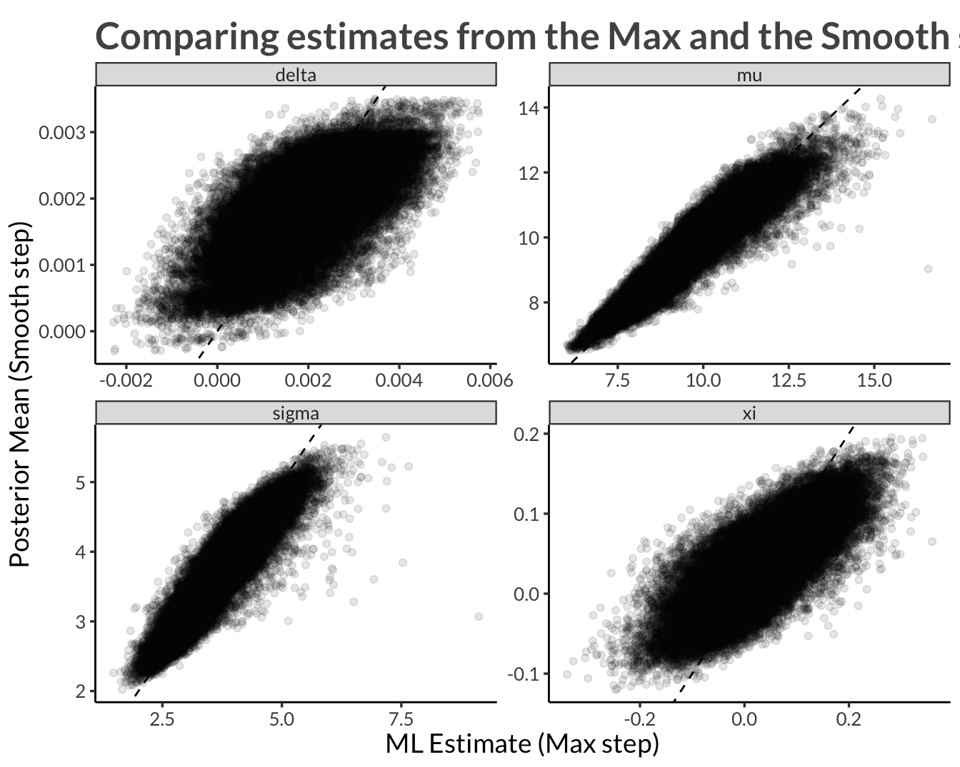
station_results |> 
  pivot_longer(c(ml_estimate, mcmc_mean)) |> 
  pivot_wider(names_from = variable) |> 
  mutate(
    mu = exp(psi),
    sigma = exp(psi + tau),
    xi = link_shape_inverse(phi),
    delta = link_trend_inverse(gamma)
  ) |> 
  select(-(gamma:tau)) |> 
  pivot_longer(c(mu:delta), names_to = "variable") |> 
  pivot_wider() |> 
  ggplot(aes(ml_estimate, mcmc_mean)) +
  geom_abline(intercept = 0, slope = 1, lty = 2) +
  geom_point(alpha = 0.1) +
  facet_wrap("variable", scales = "free") +
  labs(
    x = "ML Estimate (Max step)",
    y = "Posterior Mean (Smooth step)",
    title = "Comparing estimates from the Max and the Smooth steps"
  )

Spatial Distributions

proj_plot <- function(data) {
  
  title <- str_c(
    "Spatial distribution of estimates for ", unique(data$variable)
  )
  
  plot_dat <- data |> 
    pivot_longer(c(ml_estimate, mcmc_mean)) |> 
    mutate(
      name = fct_recode(
        factor(name),
        "Maximum Likelihood" = "ml_estimate",
        "Posterior Mean" = "mcmc_mean"
      )
    ) |> 
    group_by(name) |> 
    mutate(
      value = (value - mean(value)) / sd(value)
    ) |> 
    ungroup() |> 
    mutate(
      value = case_when(
        name == "Posterior Mean" ~ value,
        value < quantile(value, 0.0025) ~ quantile(value, 0.0025),
        value > quantile(value, 0.9975) ~ quantile(value, 0.9975),
        TRUE ~ value
      )
    )
  
  min_val <- min(plot_dat$value)
  max_val <- max(plot_dat$value)
  
  lim_range <- max(abs(min_val), abs(max_val))
  
  limits <- c(-1, 1) * lim_range
  
  plot_dat |> 
    ggplot(aes(proj_x, proj_y)) +
    geom_raster(aes(fill = value)) +
    scale_fill_viridis_c(limits = limits) +
    facet_wrap("name", nrow = 1) +
    coord_cartesian(expand = FALSE) +
    labs(
      title = title,
      fill = NULL,
      x = "X projection",
      y = "Y projection"
    )
}

Location

psi

station_results |> 
  filter(variable == "psi") |> 
  proj_plot()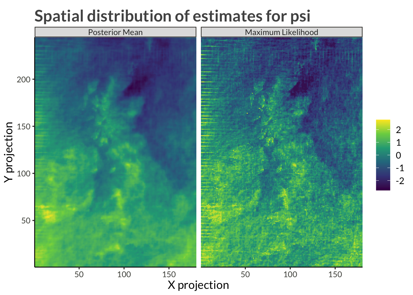

mu

station_results |> 
  filter(variable == "psi") |> 
  mutate(variable = "mu") |> 
  mutate_at(vars(ml_estimate, mcmc_mean), exp) |> 
  proj_plot()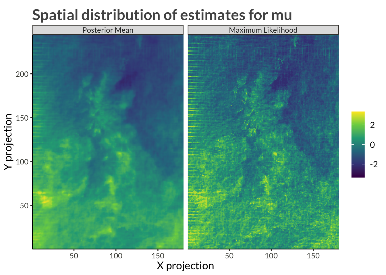

Scale

tau

station_results |> 
  filter(variable == "tau") |> 
  proj_plot()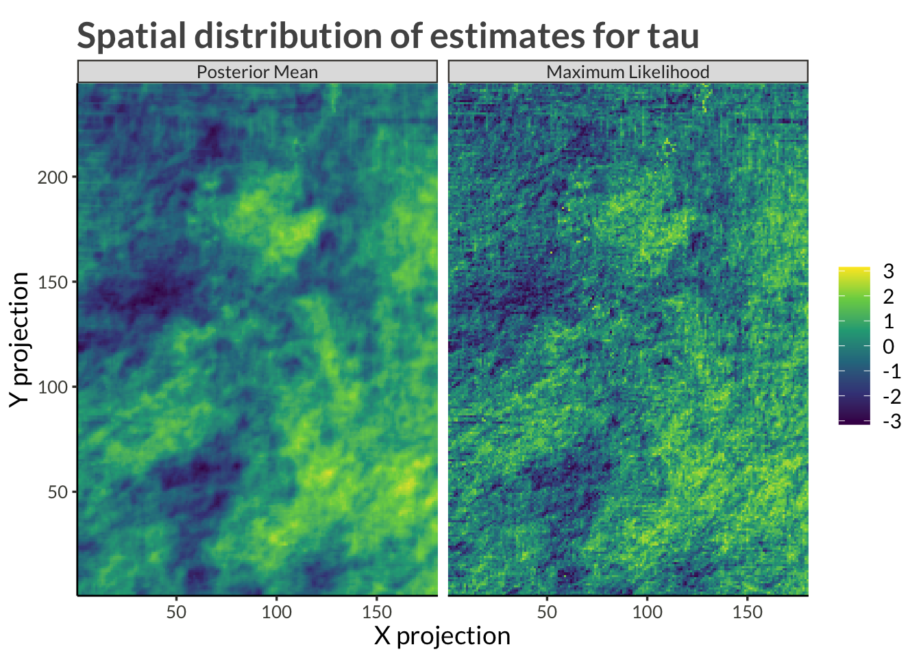

sigma

station_results |> 
  filter(variable %in% c("tau", "psi")) |> 
  pivot_longer(c(ml_estimate, mcmc_mean)) |> 
  pivot_wider(names_from = variable, values_from = value) |> 
  mutate(sigma = exp(tau + psi)) |> 
  select(-psi, -tau) |> 
  pivot_longer(c(sigma), names_to = "variable", values_to = "value") |> 
  pivot_wider() |> 
  proj_plot()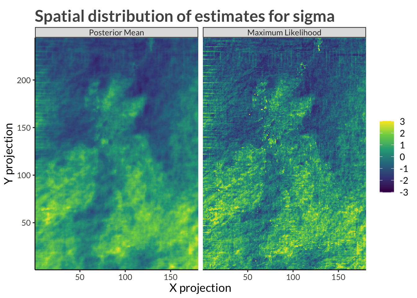

Shape

phi

station_results |> 
  filter(variable == "phi") |> 
  proj_plot()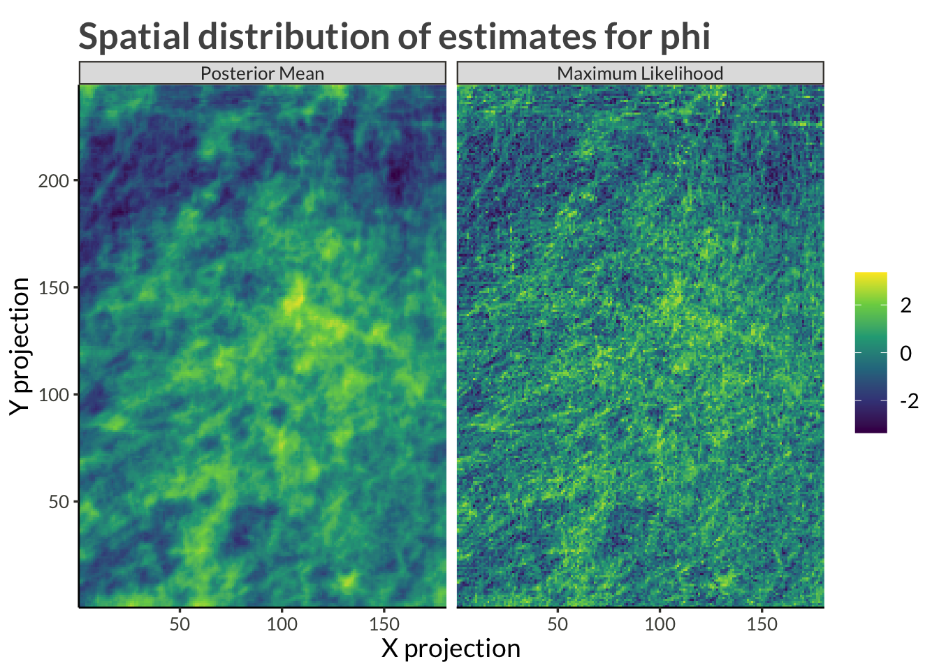

xi

station_results |> 
  filter(variable == "phi") |> 
  mutate(variable = "xi") |> 
  mutate_at(
    vars(mcmc_mean, ml_estimate),
    link_shape_inverse
  ) |> 
  proj_plot()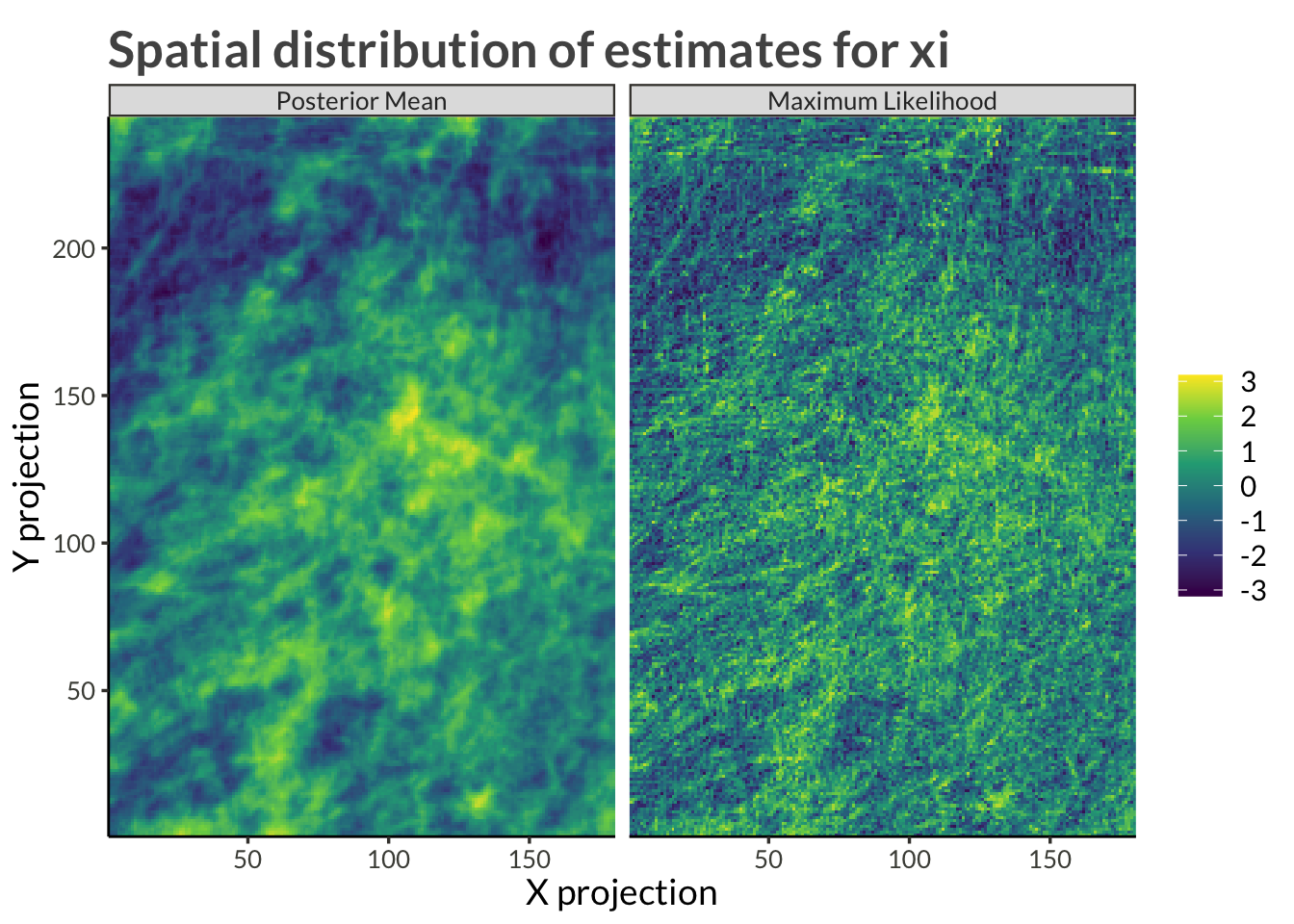

Trend

gamma

station_results |> 
  filter(variable == "gamma") |> 
  proj_plot()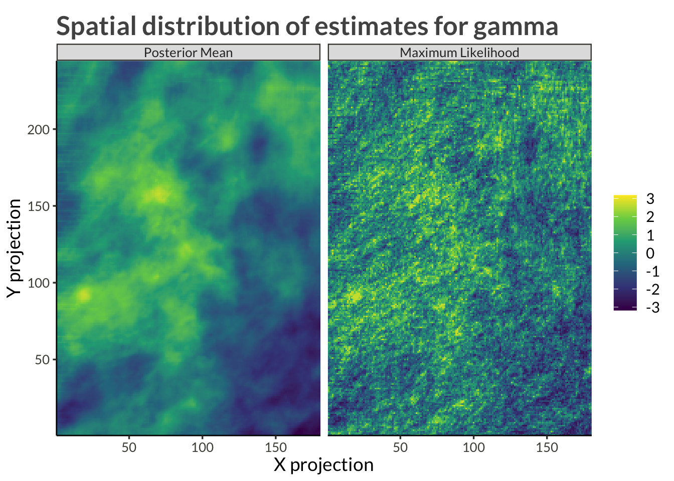

Delta

station_results |> 
  filter(variable == "gamma") |> 
  mutate(variable = "delta") |> 
  mutate_at(
    vars(mcmc_mean, ml_estimate),
    link_trend_inverse
    ) |> 
  proj_plot()