The GEV Model

In our case we want \(\mu\) to vary with time. If we write \(y_{it}\) for the observed hourly maximum at station \(i\) during year \(t\) we will then have

where

and

Maximum Likelihood Estimation

Transformed parameters

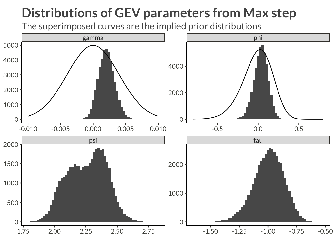
Having performed the Max step and saved the ML estimates we can easily load them by fetching the object station_estimates. Here we plot the distribution of transformed estimates.

\[\begin{aligned} \psi &= \log(\mu) \\ \tau &= \log(\frac{\sigma}{\mu}) = \log(\sigma) - \log(\mu) \\ \phi &= h(\xi) \\ \gamma &= d(\Delta), \end{aligned}\]

where the link functions for the shape and trend parameters are defined according to Johannesson et al. (2021)

Johannesson, Árni V., Stefan Siegert, Raphaël Huser, Haakon Bakka, and Birgir Hrafnkelsson. 2021. “Approximate Bayesian Inference for Analysis of Spatio-Temporal Flood Frequency Data,” April. https://doi.org/10.48550/arXiv.1907.04763.

\[\begin{aligned} h(\xi) &= a_\phi + b_\phi \log\left(-\log\left[1 - \left(\xi + \frac12\right)^{c_\phi}\right]\right) \\ c_\phi &= 0.8 \\ b_\phi &= -\frac{1}{c_\phi}\log\left(1 - \frac{1}{2^{c_\phi}}\right)\left(1 - \frac{1}{2^{c_\phi}}\right) 2^{c_\phi - 1} \\ a_\phi &= -b_\phi \log\left(-\log(1 - \frac{1}{2^{c_\phi}})\right) \\ \newline d(\Delta) &= \frac12 \delta_0 \left(\log(\delta_0 + \Delta) - \log(\delta_0 - \Delta_i)\right) \\ \delta_0 &= 0.008. \end{aligned}\]

Results

Code

library(bggjphd)
library(tidyverse)
library(GGally)
library(cowplot)
library(arrow)
library(here)
library(future)
library(progressr)
theme_set(theme_bggj())

Code

station_estimates <- read_rds("station_estimates.rds")
d <- station_estimates |> 
  select(station, par) |> 
  unnest(par) |> 
  inner_join(
    stations
  ) |> 
  select(station, proj_x, proj_y, name, value)

Distributions

Transformed Scale

Code

d_prior <- crossing(
  name = c("phi", "gamma"),
  x = seq(-1, 1, len = 200)
) |> 
  mutate(
    x = ifelse(name == "phi", x * 0.8, x * 0.01),
    y = ifelse(name == "phi", prior_shape(x) |> exp(), prior_trend(x) |> exp()),
    y = ifelse(name == "phi", y * 6000, y * 0.05)
  )


d |> 
  ggplot(aes(value)) +
  geom_histogram(bins = 60) +
  geom_line(
    data = d_prior,
    aes(x = x, y = y * 1e3),
    inherit.aes = F
  ) +
  facet_wrap("name", scales = "free") +
  labs(
    x = NULL,
    y = NULL,
    title = "Distributions of GEV parameters from Max step",
    subtitle = "The superimposed curves are the implied prior distributions"
  )

Code

d |> 
  pivot_wider() |> 
  select(-station, -proj_x, -proj_y) |> 
  ggpairs(progress = FALSE)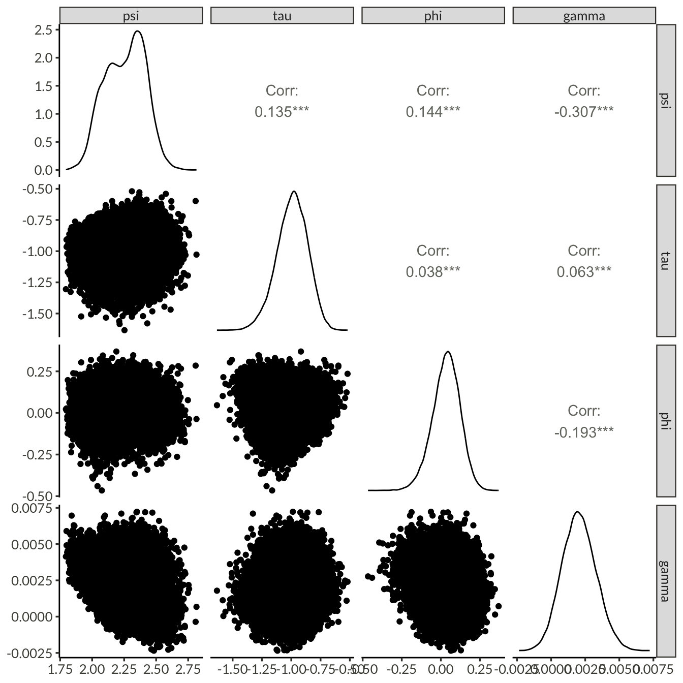

Original Scale

Code

d_prior <- crossing(
  name = c("phi", "gamma"),
  x = seq(-1, 1, len = 200)
) |> 
  mutate(
    x = ifelse(name == "phi", x * 0.8, x * 0.01),
    y = ifelse(name == "phi", prior_shape(x) |> exp(), prior_trend(x) |> exp()),
    y = ifelse(name == "phi", y * 2000000, y * 20),
    x = ifelse(name == "phi", link_shape_inverse(x), link_trend_inverse(x)),
    name = ifelse(name == "phi", "xi", "delta")
  )

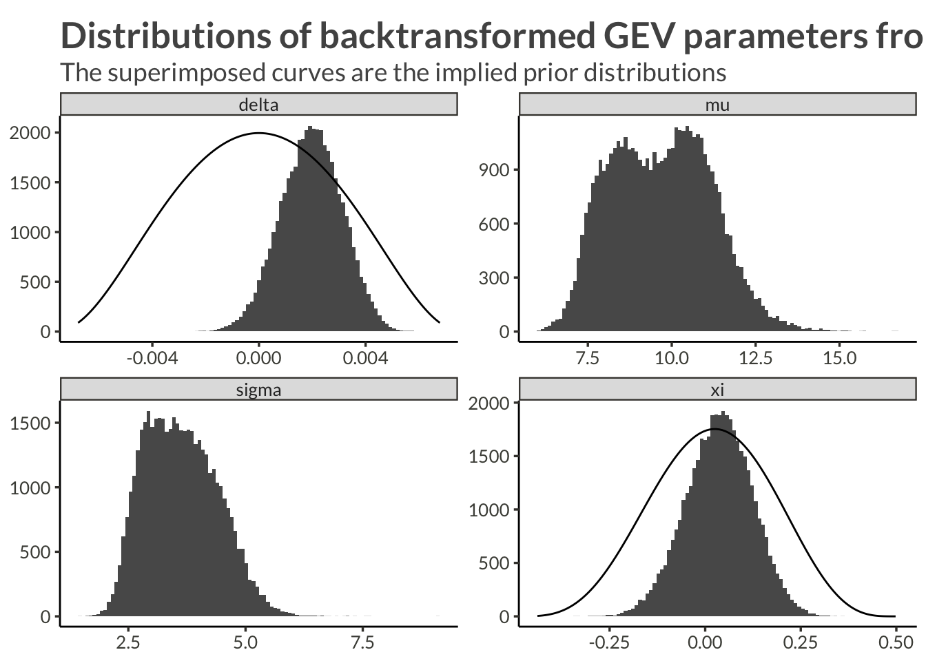
d |> 
  pivot_wider() |> 
  mutate(mu = exp(psi),
         sigma = exp(tau + psi),
         xi = link_shape_inverse(phi),
         delta = link_trend_inverse(gamma)) |> 
  select(-psi, -tau, -phi, -gamma, -proj_x, -proj_y) |> 
  pivot_longer(c(-station)) |> 
  mutate(name = fct_relevel(name, "mu", "sigma", "xi", "delta")) |> 
  ggplot(aes(value)) +
  geom_histogram(bins = 100) +
  geom_line(
    data = d_prior,
    aes(x = x, y = y),
    inherit.aes = F
  ) +
  facet_wrap("name", scales = "free") +
  labs(
    x = NULL,
    y = NULL,
    title = "Distributions of backtransformed GEV parameters from Max step",
    subtitle = "The superimposed curves are the implied prior distributions"
  )

Code

d |> 
  pivot_wider() |> 
  mutate(mu = exp(psi),
         sigma = exp(tau + psi),
         xi = link_shape_inverse(phi),
         delta = link_trend_inverse(gamma)) |> 
  select(-psi, -tau, -phi, -gamma, -station, -proj_x, -proj_y) |> 
  ggpairs(progress = FALSE)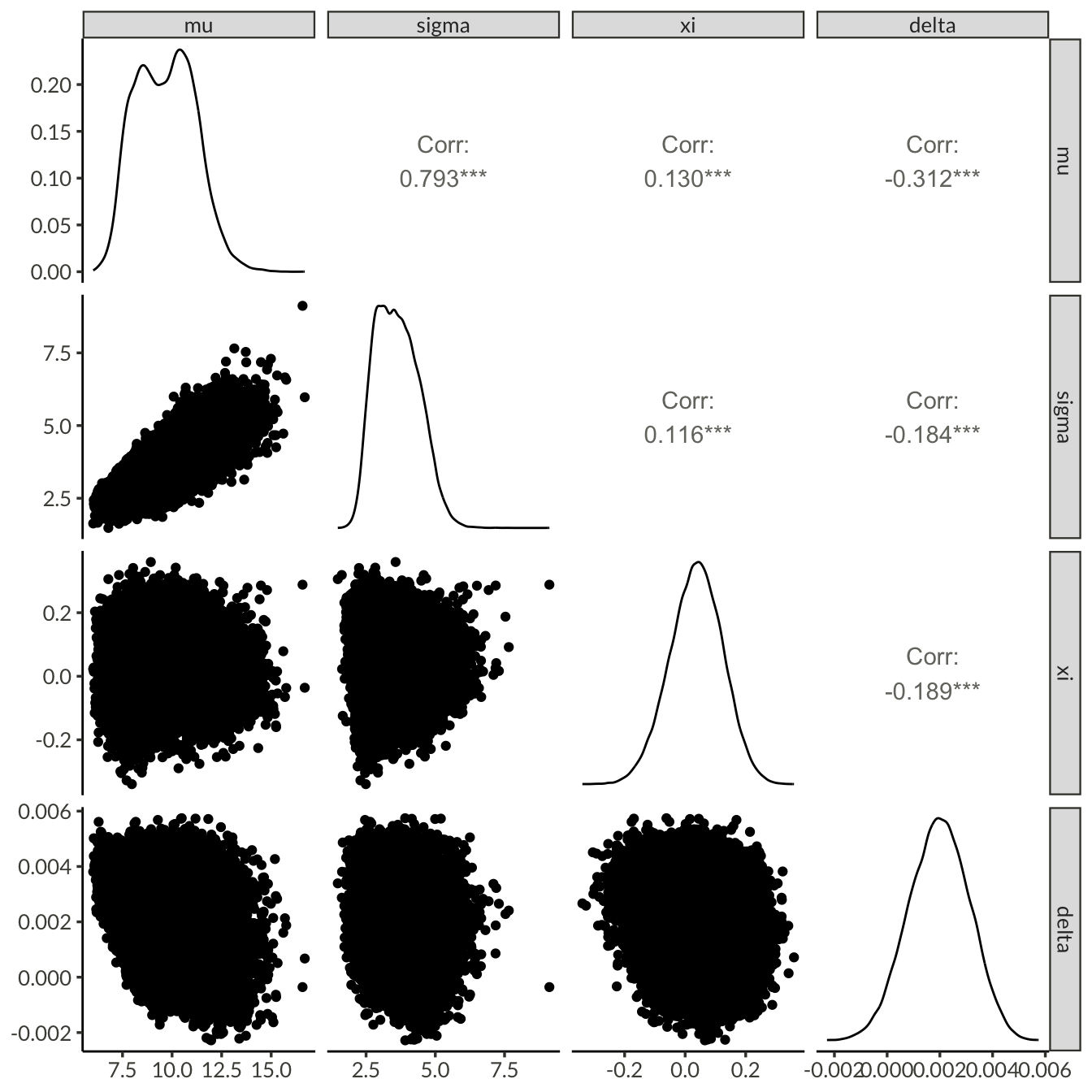

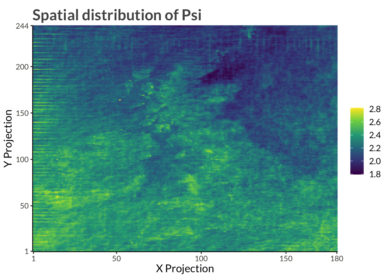
Spatial Distribution

Location

Code

d |> 
  filter(name == "psi") |> 
  ggplot(aes(proj_x, proj_y, fill = value)) +
  geom_raster(interpolate = TRUE) +
  scale_x_continuous(
    expand = expansion(),
    breaks = c(range(d$proj_x), pretty(d$proj_x))
  ) +
  scale_y_continuous(
    expand = expansion(),
    breaks = c(range(d$proj_y), pretty(d$proj_y))
  ) +
  scale_fill_viridis_c() +
  labs(
    x = "X Projection",
    y = "Y Projection",
    fill = NULL,
    title = "Spatial distribution of Psi"
  )

Code

d |> 
  filter(name == "psi") |> 
  ggplot(aes(proj_x, proj_y, fill = exp(value))) +
  geom_raster(interpolate = TRUE) +
  scale_x_continuous(
    expand = expansion(),
    breaks = c(range(d$proj_x), pretty(d$proj_x))
  ) +
  scale_y_continuous(
    expand = expansion(),
    breaks = c(range(d$proj_y), pretty(d$proj_y))
  ) +
  scale_fill_viridis_c() +
  labs(
    x = "X Projection",
    y = "Y Projection",
    fill = NULL,
    title = "Spatial distribution of Mu"
  )

Scale

Code

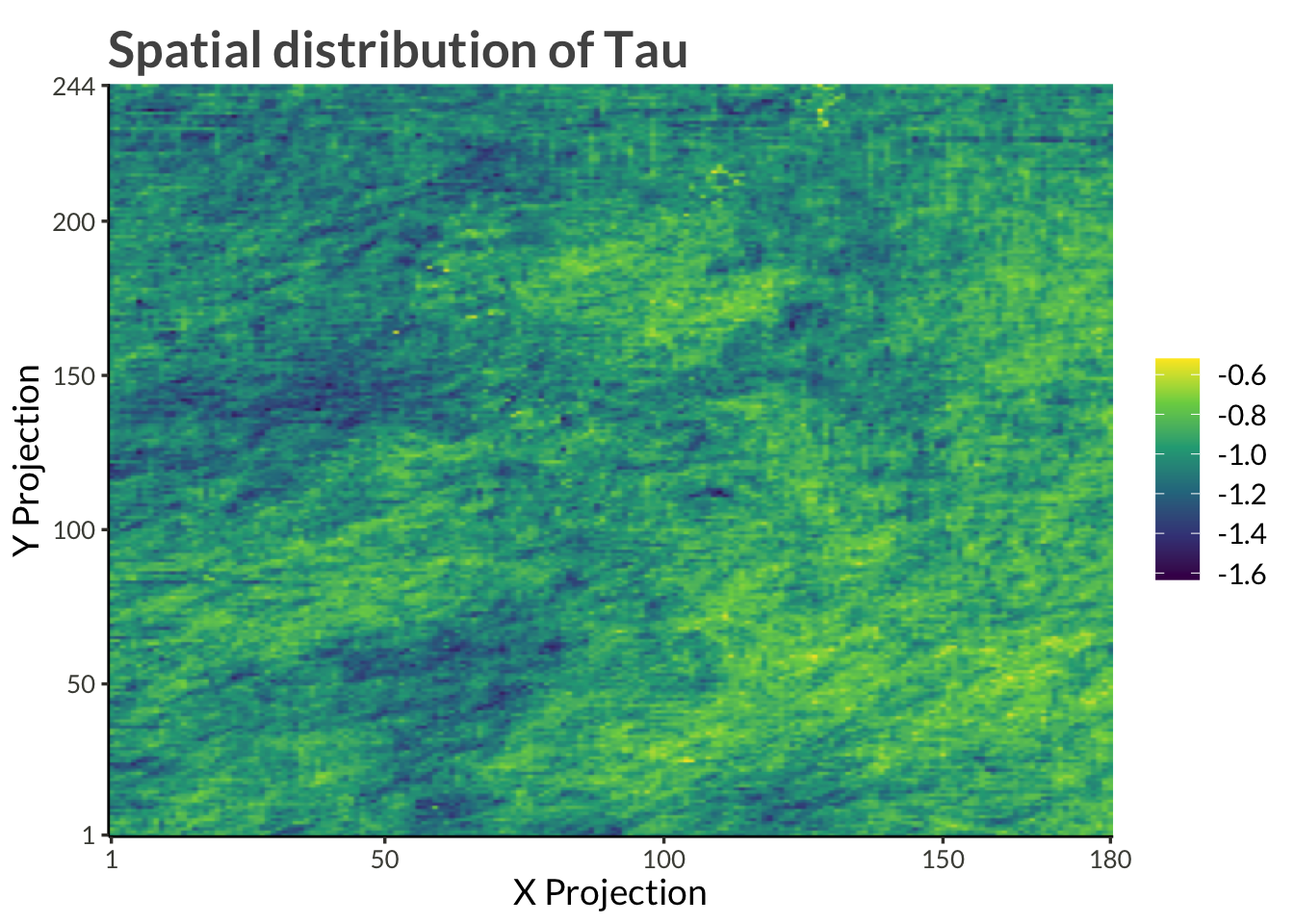
d |> 
  filter(name == "tau") |> 
  ggplot(aes(proj_x, proj_y, fill = value)) +
  geom_raster(interpolate = TRUE) +
  scale_x_continuous(
    expand = expansion(),
    breaks = c(range(d$proj_x), pretty(d$proj_x))
  ) +
  scale_y_continuous(
    expand = expansion(),
    breaks = c(range(d$proj_y), pretty(d$proj_y))
  ) +
  scale_fill_viridis_c() +
  labs(
    x = "X Projection",
    y = "Y Projection",
    fill = NULL,
    title = "Spatial distribution of Tau"
  )

Code

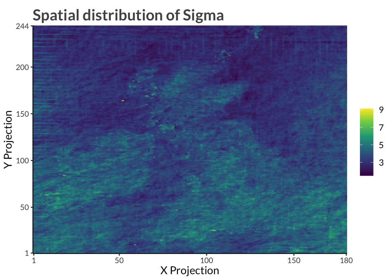
d |> 
  pivot_wider() |> 
  mutate(sigma = exp(tau + psi)) |> 
  ggplot(aes(proj_x, proj_y, fill = sigma)) +
  geom_raster(interpolate = TRUE) +
  scale_x_continuous(
    expand = expansion(),
    breaks = c(range(d$proj_x), pretty(d$proj_x))
  ) +
  scale_y_continuous(
    expand = expansion(),
    breaks = c(range(d$proj_y), pretty(d$proj_y))
  ) +
  scale_fill_viridis_c() +
  labs(
    x = "X Projection",
    y = "Y Projection",
    fill = NULL,
    title = "Spatial distribution of Sigma"
  )

Shape

Code

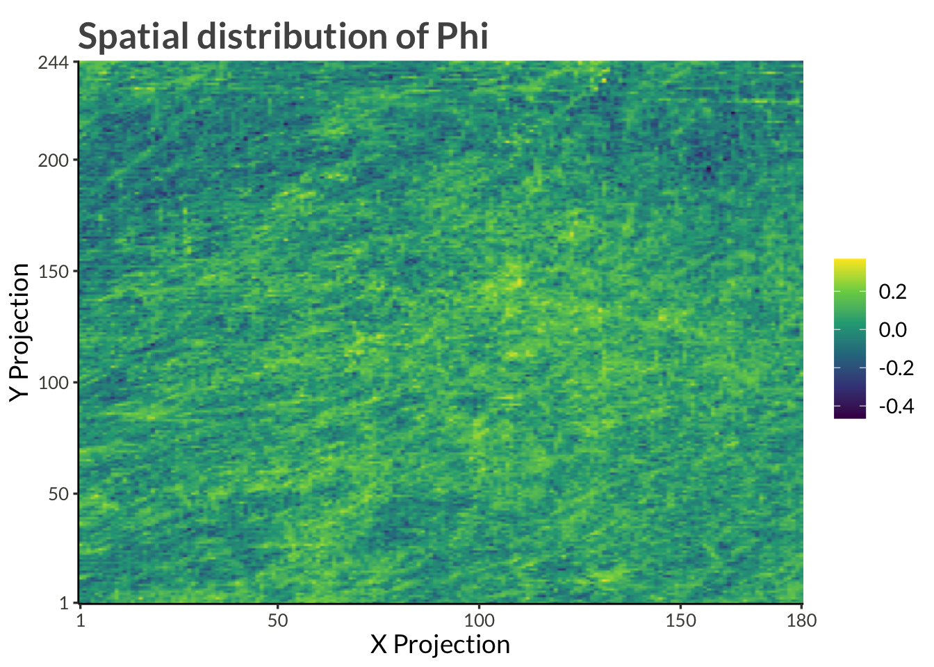
d |> 
  filter(name == "phi") |> 
  ggplot(aes(proj_x, proj_y, fill = value)) +
  geom_raster(interpolate = TRUE) +
  scale_x_continuous(
    expand = expansion(),
    breaks = c(range(d$proj_x), pretty(d$proj_x))
  ) +
  scale_y_continuous(
    expand = expansion(),
    breaks = c(range(d$proj_y), pretty(d$proj_y))
  ) +
  scale_fill_viridis_c() +
  labs(
    x = "X Projection",
    y = "Y Projection",
    fill = NULL,
    title = "Spatial distribution of Phi"
  )

Code

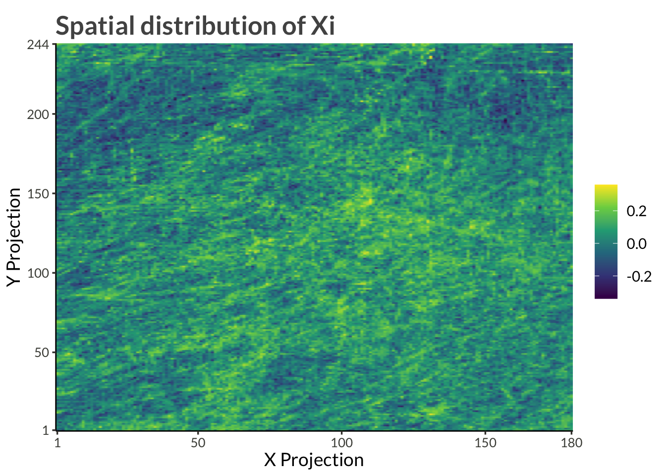
d |> 
  pivot_wider() |> 
  mutate(xi = link_shape_inverse(phi)) |> 
  ggplot(aes(proj_x, proj_y, fill = xi)) +
  geom_raster(interpolate = TRUE) +
  scale_x_continuous(
    expand = expansion(),
    breaks = c(range(d$proj_x), pretty(d$proj_x))
  ) +
  scale_y_continuous(
    expand = expansion(),
    breaks = c(range(d$proj_y), pretty(d$proj_y))
  ) +
  scale_fill_viridis_c() +
  labs(
    x = "X Projection",
    y = "Y Projection",
    fill = NULL,
    title = "Spatial distribution of Xi"
  )

Trend

Code

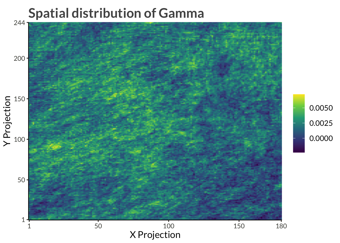
d |> 
  filter(name == "gamma") |> 
  ggplot(aes(proj_x, proj_y, fill = value)) +
  geom_raster(interpolate = TRUE) +
  scale_x_continuous(
    expand = expansion(),
    breaks = c(range(d$proj_x), pretty(d$proj_x))
  ) +
  scale_y_continuous(
    expand = expansion(),
    breaks = c(range(d$proj_y), pretty(d$proj_y))
  ) +
  scale_fill_viridis_c() +
  labs(
    x = "X Projection",
    y = "Y Projection",
    fill = NULL,
    title = "Spatial distribution of Gamma"
  )

Code

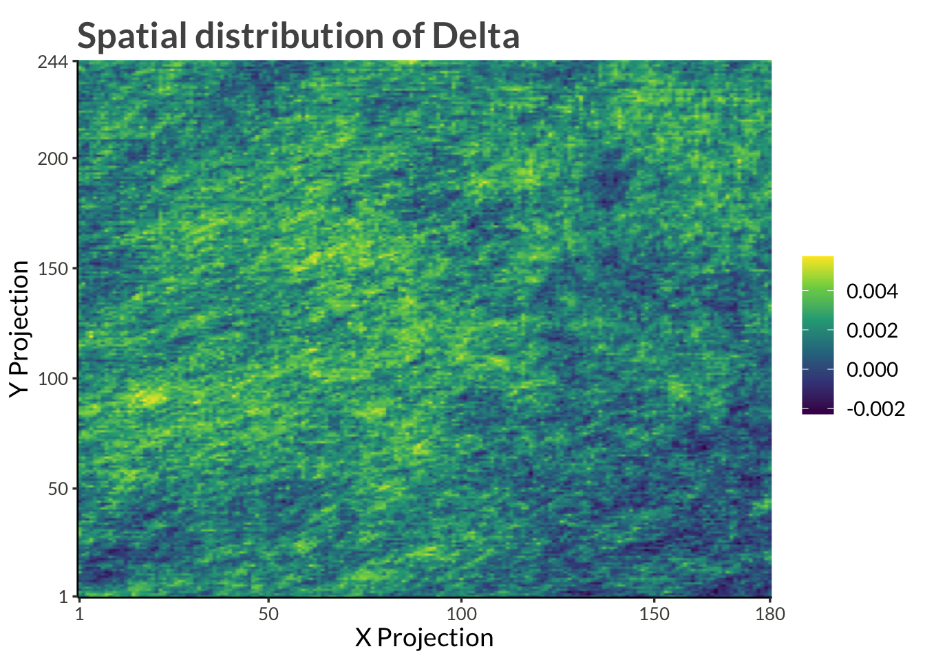
d |> 
  pivot_wider() |> 
  mutate(delta = link_trend_inverse(gamma)) |> 
  ggplot(aes(proj_x, proj_y, fill = delta)) +
  geom_raster(interpolate = TRUE) +
  scale_x_continuous(
    expand = expansion(),
    breaks = c(range(d$proj_x), pretty(d$proj_x))
  ) +
  scale_y_continuous(
    expand = expansion(),
    breaks = c(range(d$proj_y), pretty(d$proj_y))
  ) +
  scale_fill_viridis_c() +
  labs(
    x = "X Projection",
    y = "Y Projection",
    fill = NULL,
    title = "Spatial distribution of Delta"
  )

Fit

Code

pgev <- function(y, loc, scale, shape) {
  out <- 1 + shape * (y - loc) / scale
  out <- out ^ (-1/shape)
  out <- exp(-out)
  out
}

Code

plot_dat <- d |> 
  pivot_wider(names_from = name, values_from = value) |>
  mutate(
    mu0 = exp(psi),
    sigma = exp(tau + psi),
    xi = link_shape_inverse(phi),
    delta = link_trend_inverse(gamma)
  ) |> 
  select(-(psi:gamma)) |> 
  inner_join(
    precip,
    by = join_by(station), 
    multiple = "all"
  ) |> 
  mutate(
    mu = mu0 * (1 + delta * (year - 1981)),
    p = pgev(precip, mu, sigma, xi)
  ) |> 
  arrange(station, (precip - mu)) |> 
  select(station, year, precip, p) |> 
  mutate(
    q = row_number() / (n() + 1),
    station_diff = sqrt(mean((p - q)^2)),
    .by = station
  ) |> 
  mutate(
    year_diff = sqrt(mean((p - q)^2)),
    .by = year
  )

Code

plot_dat |>
  nest(data = -c(station, station_diff)) |> 
  arrange(desc(station_diff)) |> 
  slice(1:9) |> 
  unnest(data) |> 
  ggplot(aes(p, q)) +
  geom_abline(intercept = 0, slope = 1, lty = 2) +
  geom_line() +
  facet_wrap("station")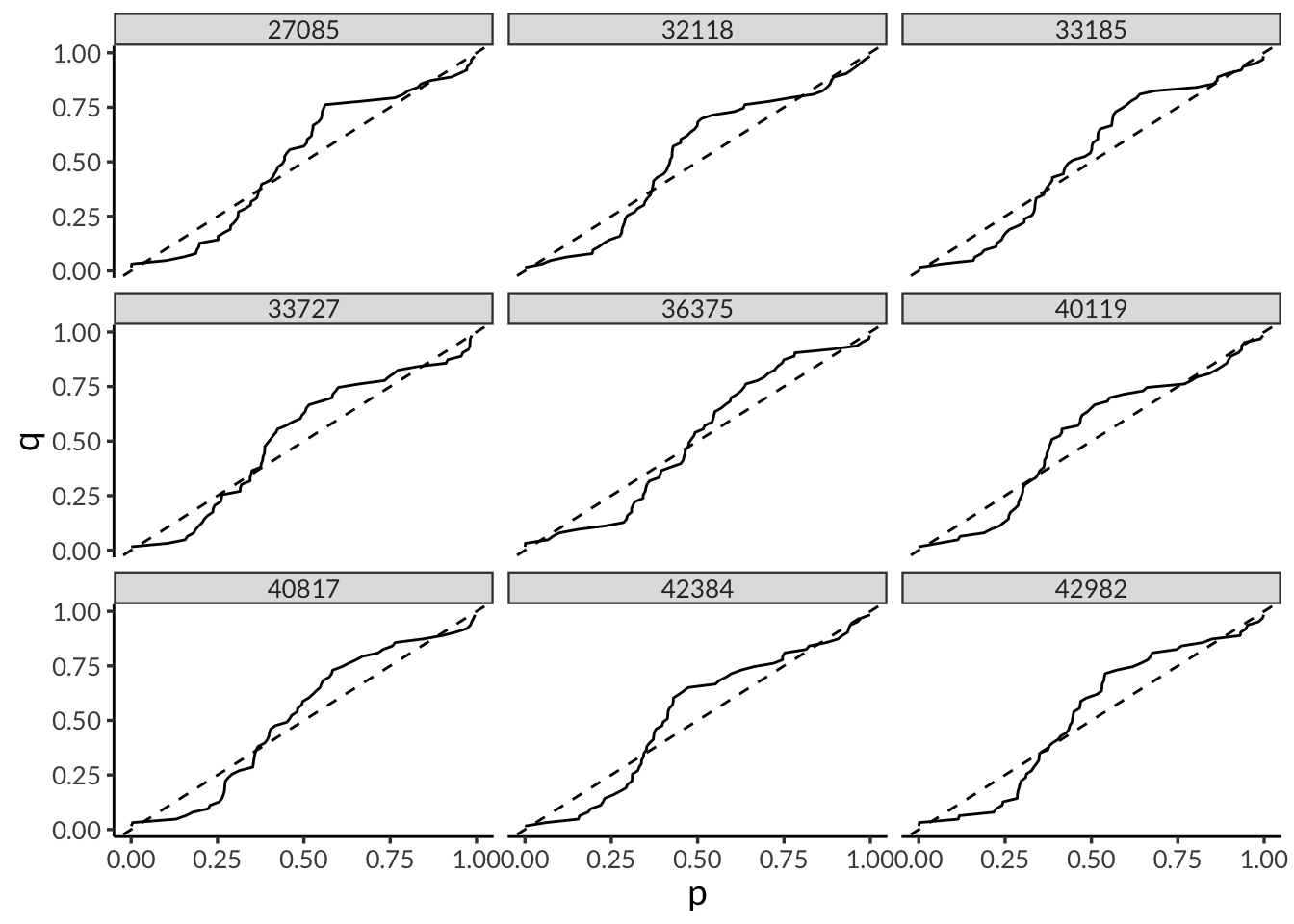

Code

plot_dat |>
  nest(data = -c(station, station_diff)) |> 
  arrange(station_diff) |> 
  slice(1:9) |> 
  unnest(data) |> 
  ggplot(aes(p, q)) +
  geom_abline(intercept = 0, slope = 1, lty = 2) +
  geom_line() +
  facet_wrap("station")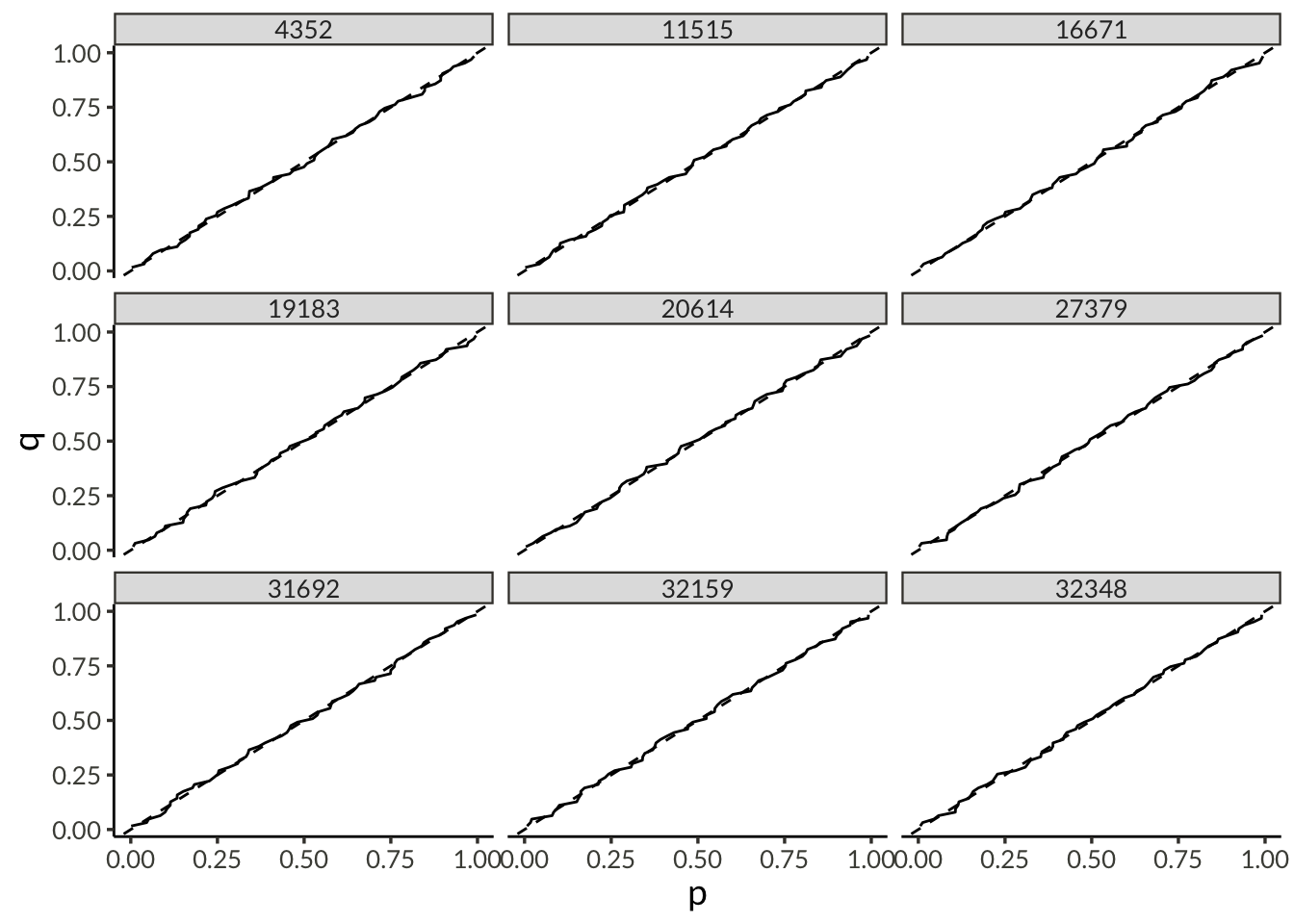

Code

plot_dat |> 
  distinct(station, station_diff) |> 
  inner_join(
    stations
  ) |> 
  ggplot(aes(proj_x, proj_y, fill = station_diff)) +
  geom_raster() +
  scale_fill_viridis_c() +
  coord_cartesian(expand = FALSE)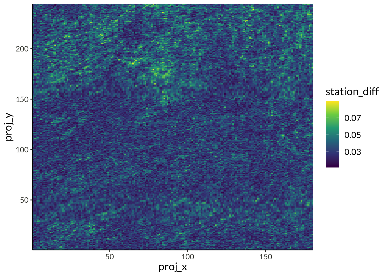

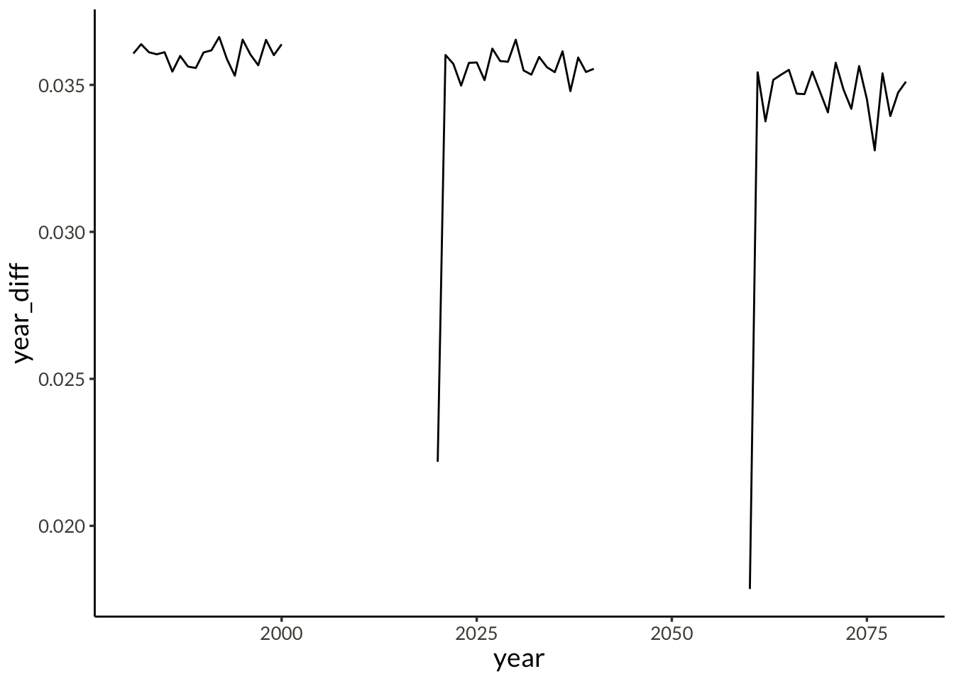
Code

plot_dat |> 
  distinct(year, year_diff) |> 
  mutate(
    period = case_when(
      year < 2020 ~ 1,
      year < 2060 ~ 2,
      TRUE ~ 3
    )
  ) |> 
  ggplot(aes(year, year_diff, group = period)) +
  geom_line()