T-Copula

Code
library(bggjphd)
library(tidyverse)
library(progressr)
library(future)
library(bayesplot)
library(GGally)
library(scales)
library(cowplot)
library(kableExtra)
library(arrow)
library(tictoc)
library(broom)
library(corrr)
library(patchwork)
theme_set(theme_half_open())

Summary

At this point we have performed the Max-and-Smooth estimation procedure and obtained samples from the posterior distribution of the location-wise GEV parameters.

In this analysis we

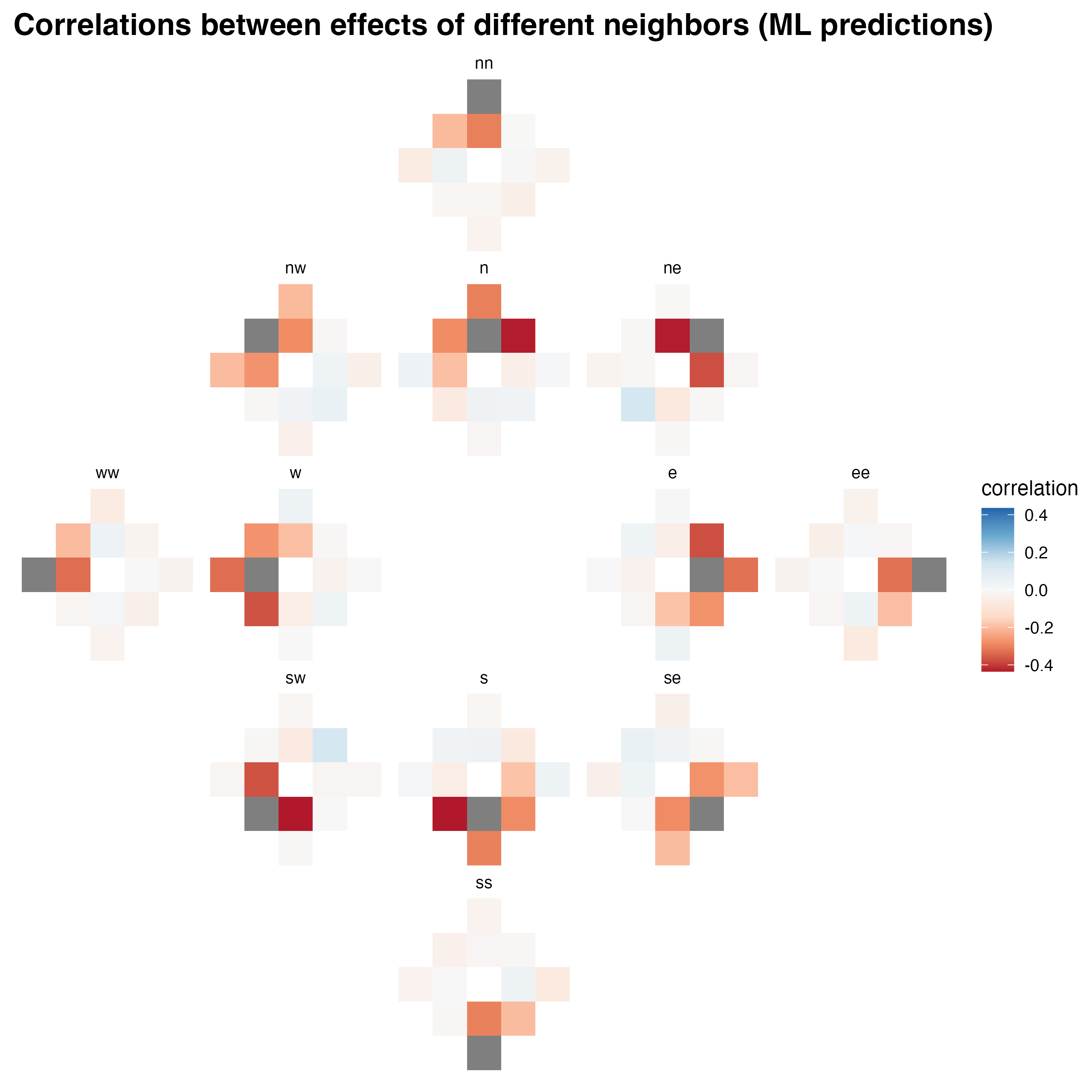
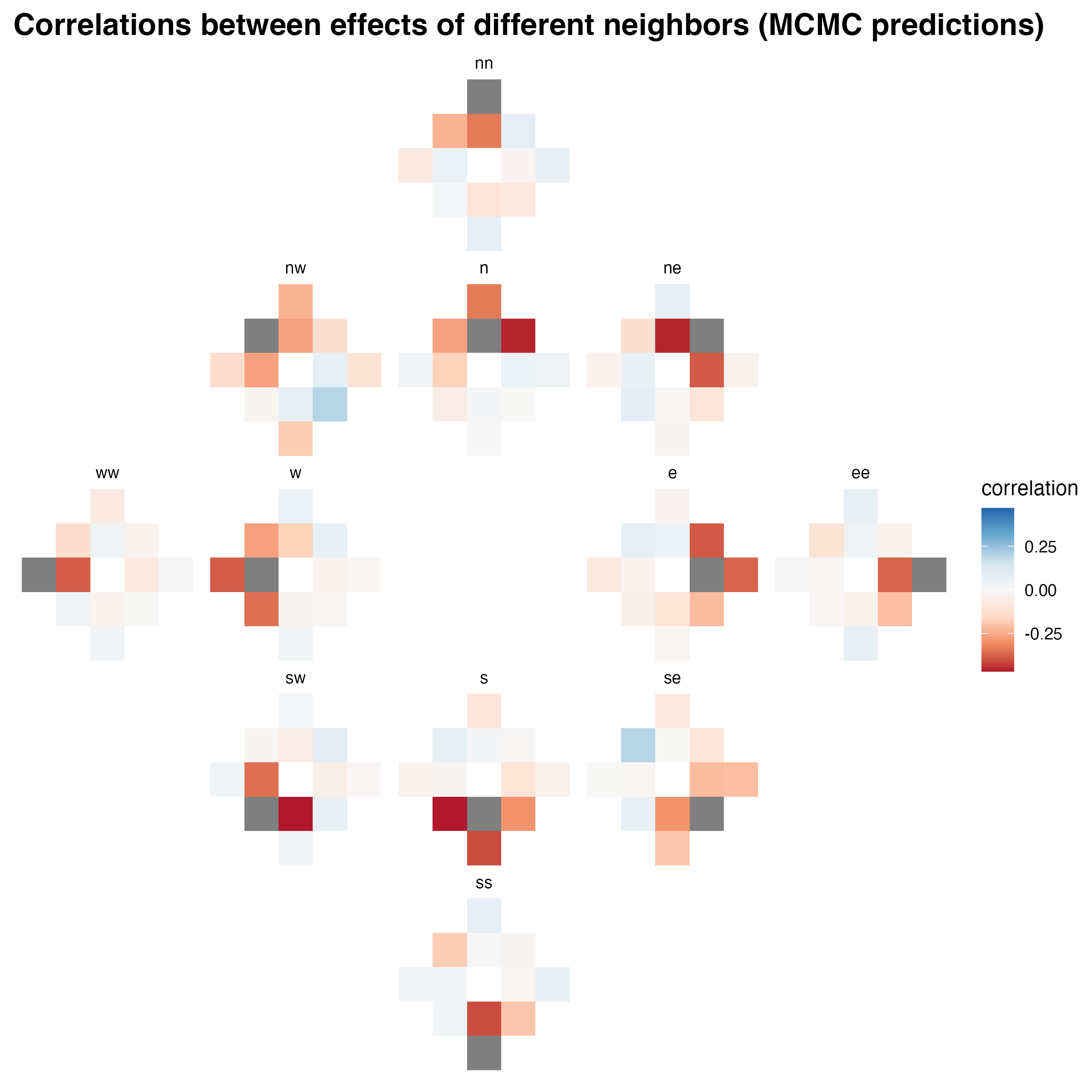
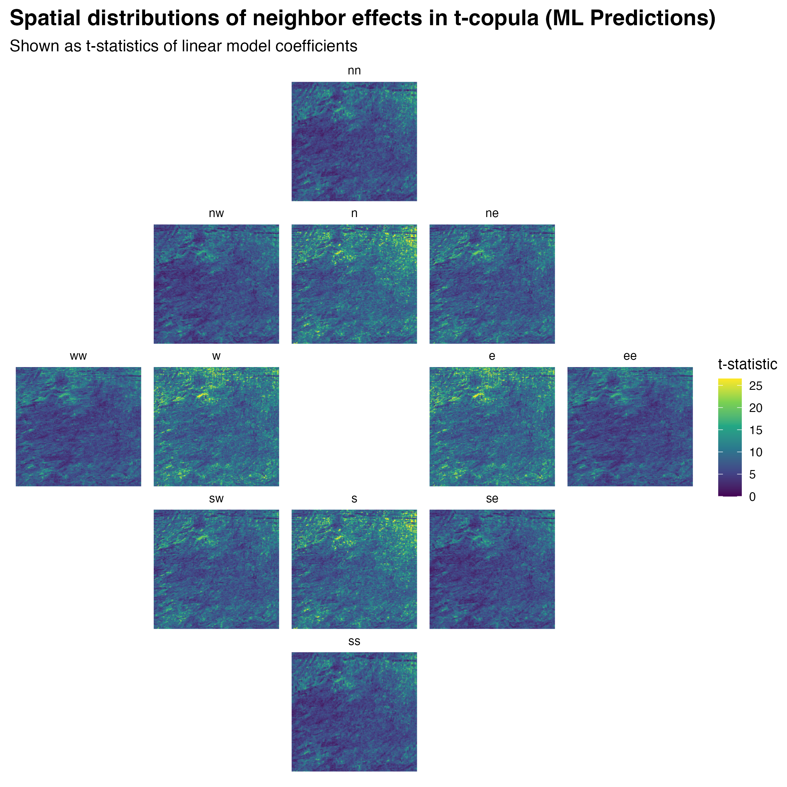
  • use these estimates to obtain posterior predictions of the observed extreme precipitation observations in the form of probability values in the range (0, 1).
  • We then convert these probabilities into t-distributed observations by using the quantile function of the t-distribution with mean 0, variance 1 and degrees-of-freedom 3.
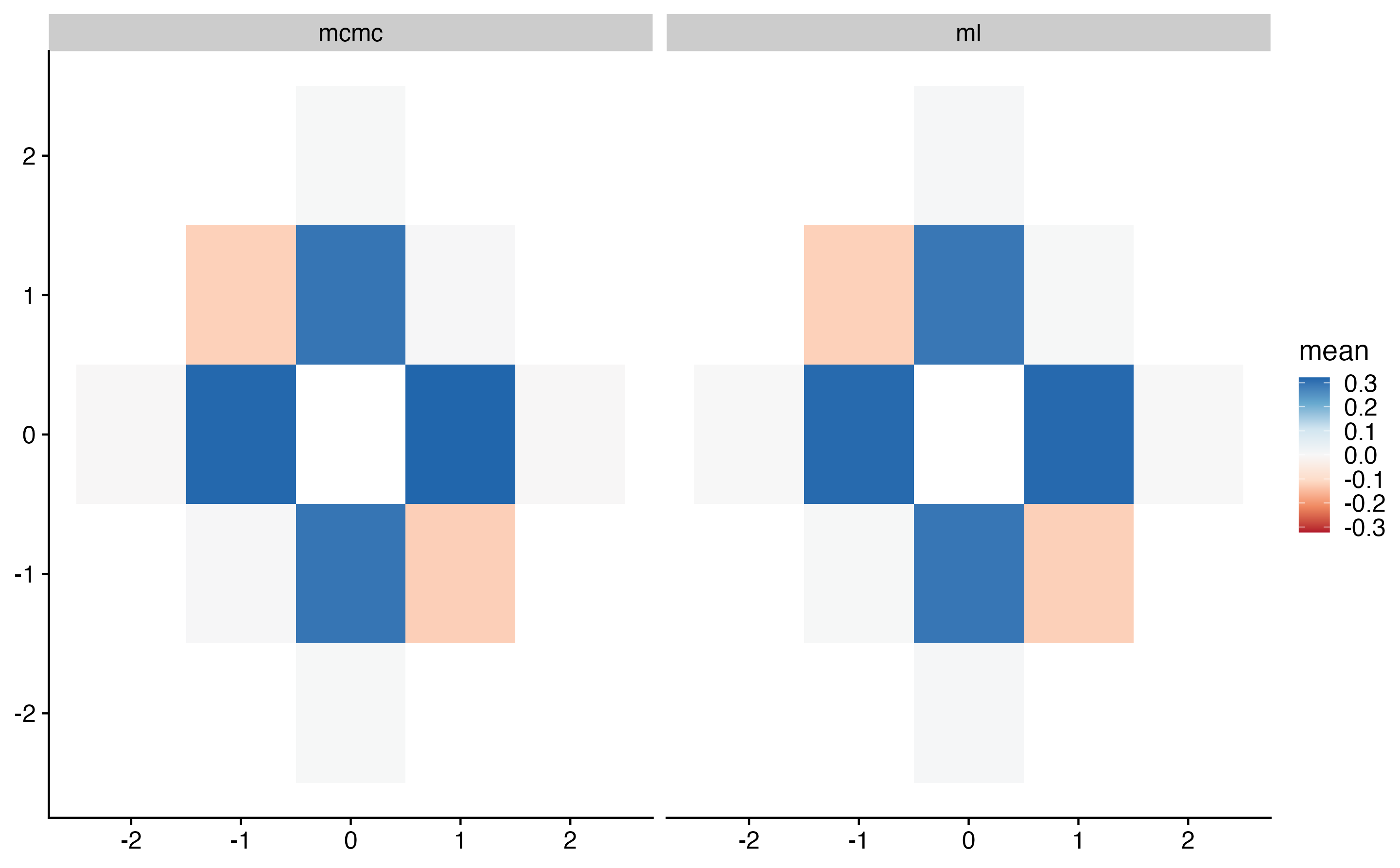
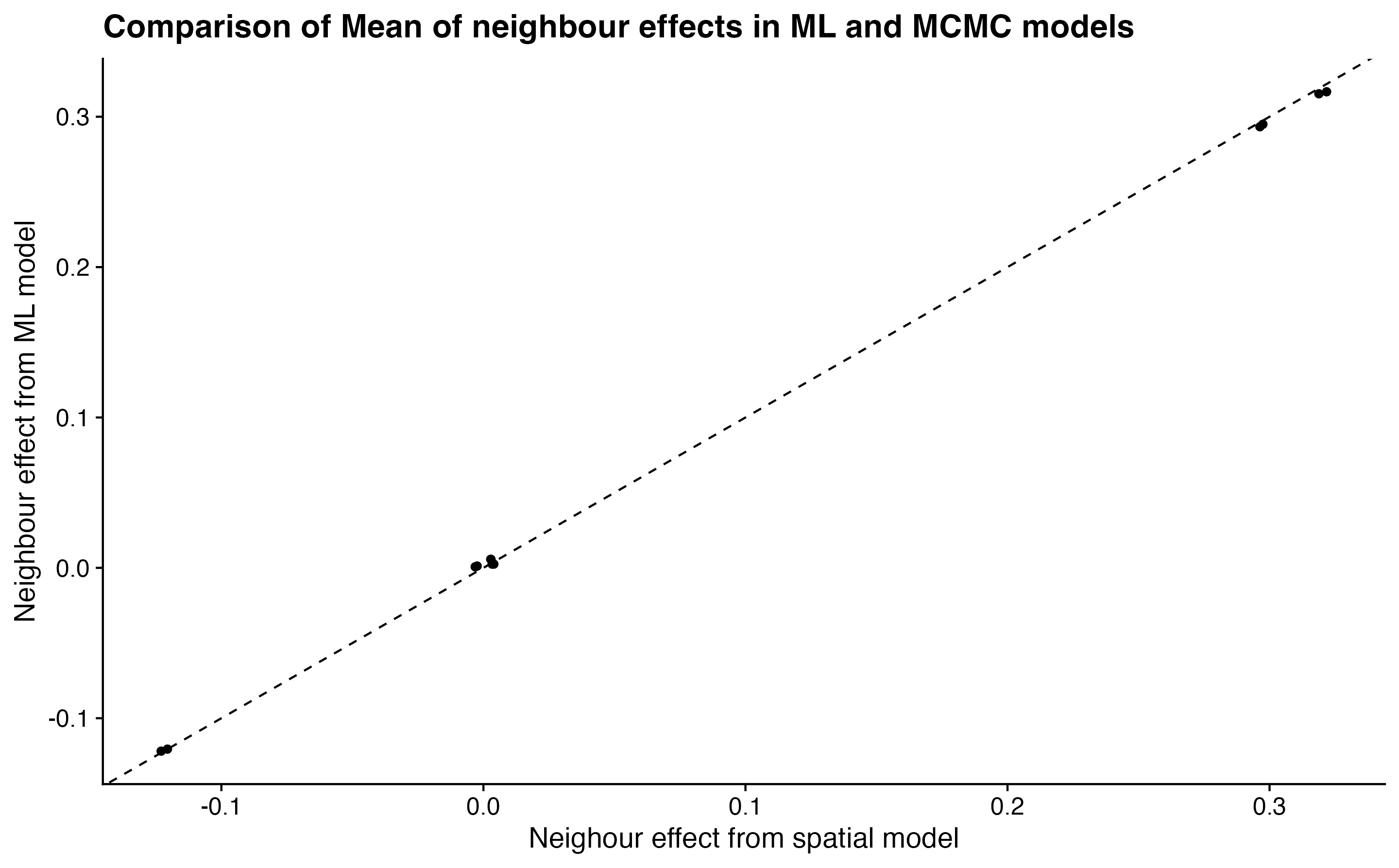
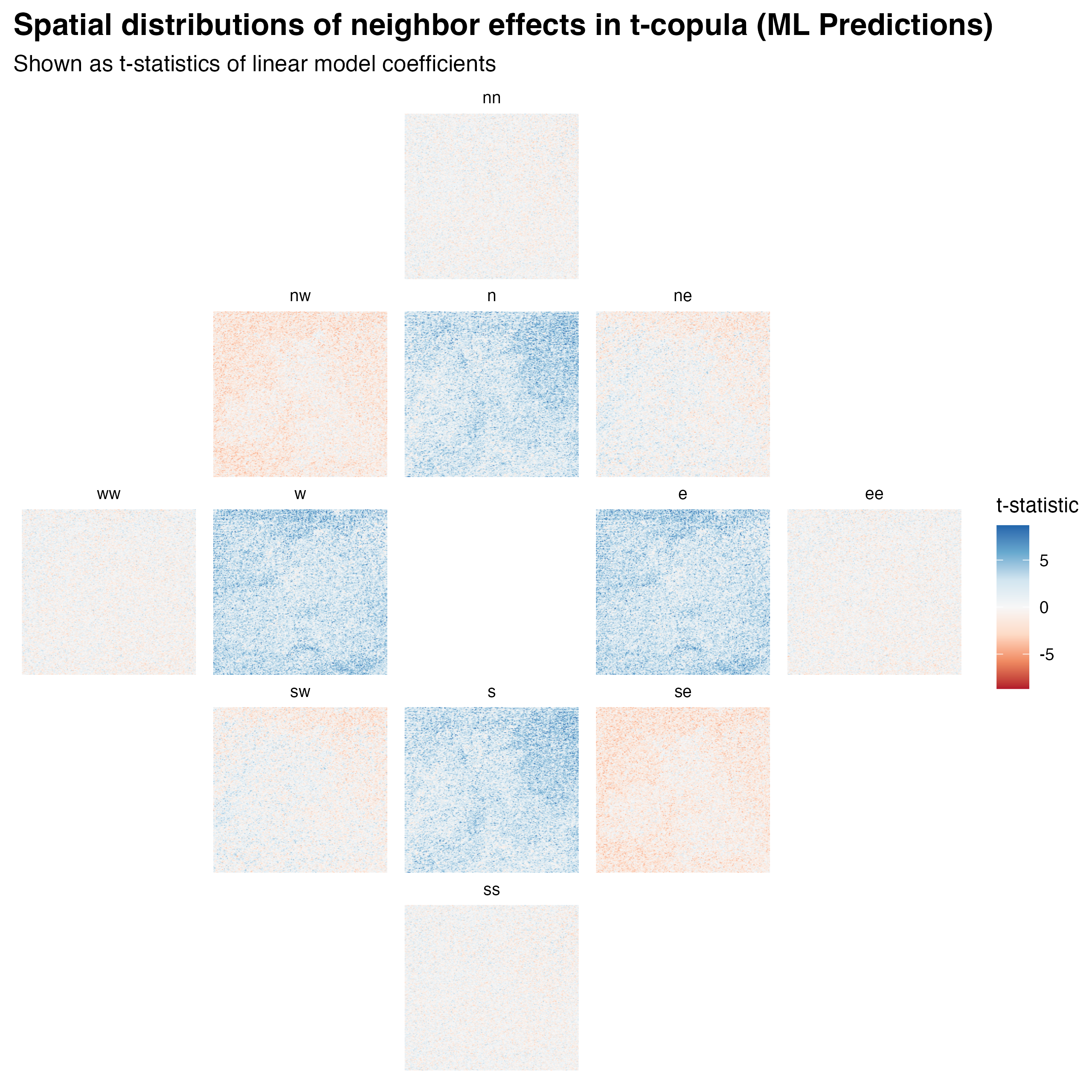
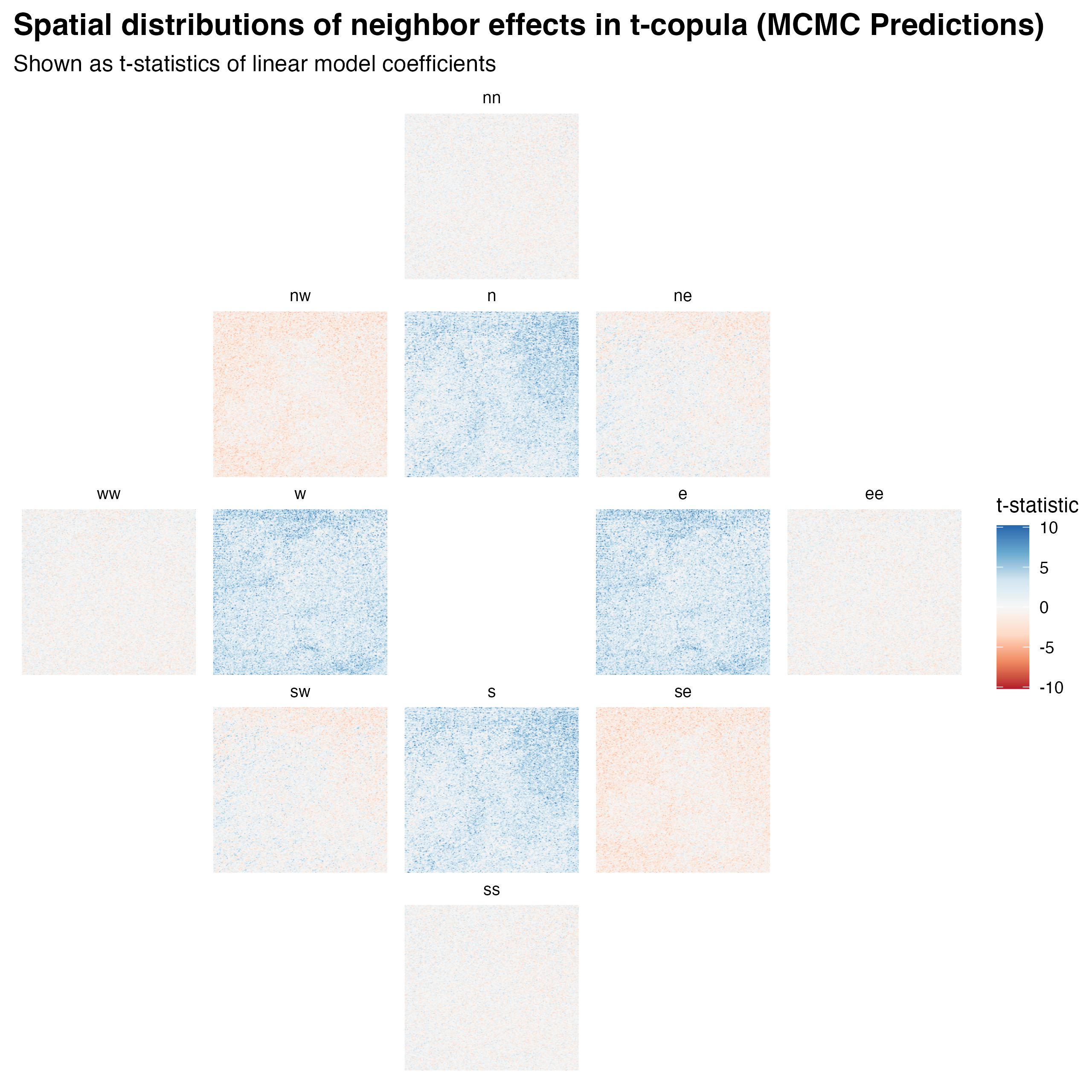
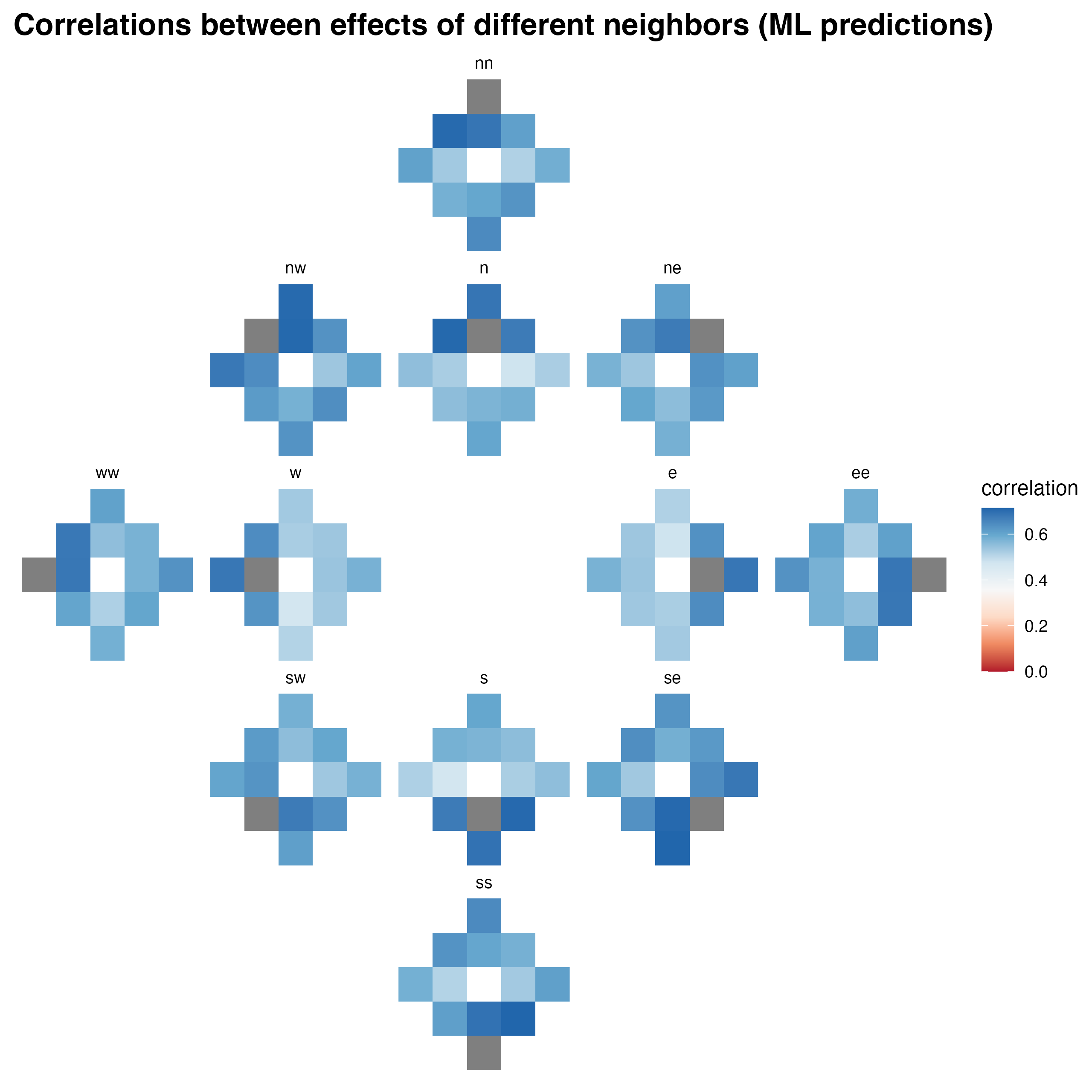
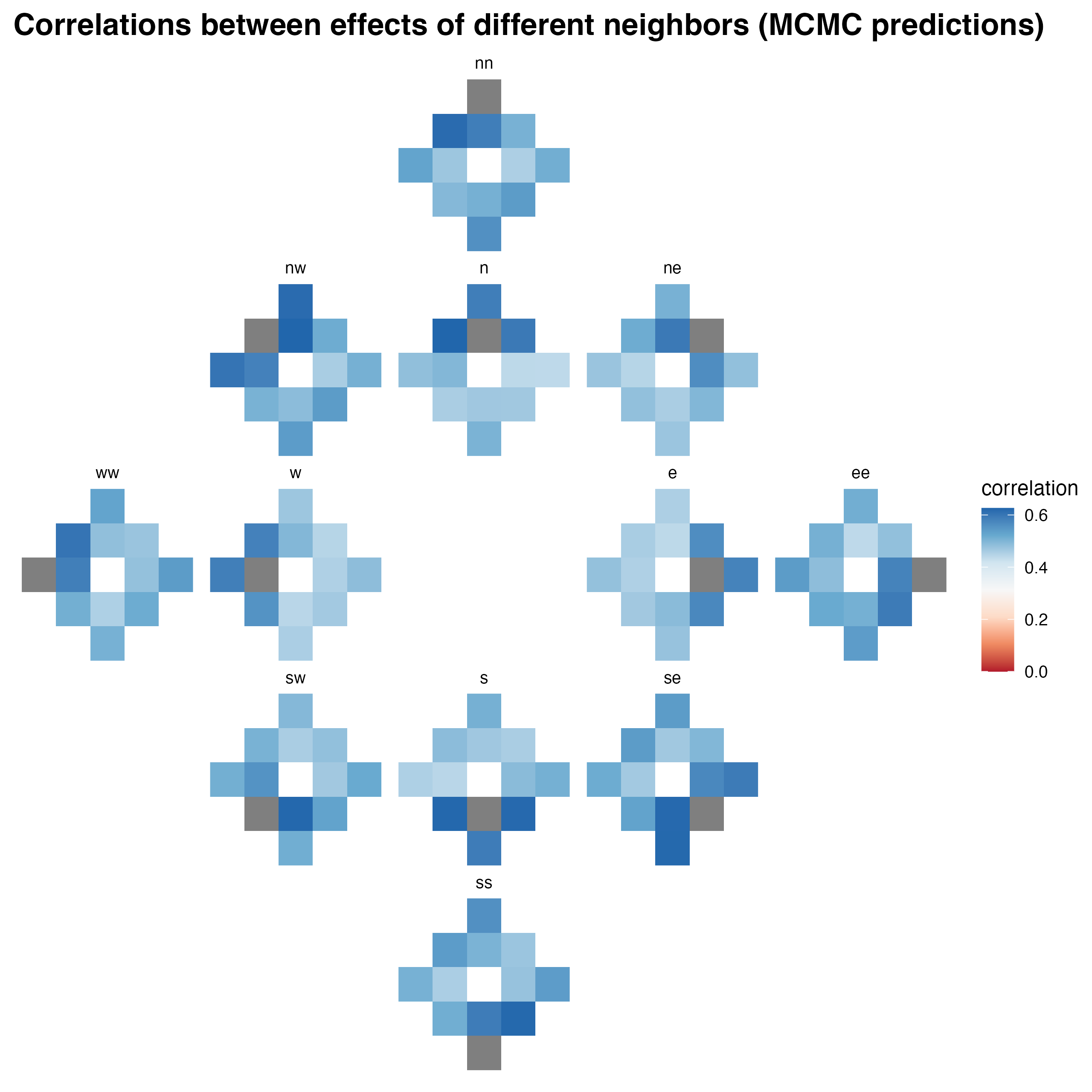
  • Using these t-distributed variables we want to find out how much the observed discrepancies are correlated with the discrepancies of a location’s neighbors
Code
b <- -log(1 - (1/2)^0.5) * (1 - (1/2)^0.5) * 2^(0.5 - 1) / 0.5
a <- -b * log(-log(1 - (1/2)^0.5))

pgev <- function(y, loc, scale, shape) {
  out <- 1 + shape * (y - loc) / scale
  out <- out ^ (-1/shape)
  out <- exp(-out)
  out
} 

#| eval: false
mcmc <- open_dataset("data/posterior_samples.parquet") |> 
  to_duckdb()

i <- c(0, seq_len(floor(nrow(stations) / 100)))

get_t_vals <- function(idx) {
  gc()
  Sys.sleep(0.1)
  out <- mcmc |> 
    filter(floor(station/100) == idx) |> 
    mutate(
      mu = exp(psi),
      sigma = exp(psi + tau),
      xi =  (1 - exp(-exp((phi - a)/b))) ^ (1 / 0.5) - 1/2,
      delta = 0.008 * (exp(2 * gamma / 0.008) - 1) / (exp(2 * gamma / 0.008) + 1)
    ) |> 
    select(chain, iter, station, mu0 = mu, sigma, xi, delta) |> 
    collect() |> 
    inner_join(
      precip,
      by = "station"
    ) |> 
    mutate(
      mu = mu0 * (1 + delta * (year - 1981)),
      p = pgev(precip, mu, sigma, xi),
      t_val = qt(p = p, df = 3)
    ) |> 
    summarise(
      t_val = mean(t_val, na.rm = TRUE),
      .by = c(station, year, precip)
    )
  
  out
}

mcmc_results <- map_dfr(
  i, 
  get_t_vals
)

ml_results <- station_estimates |> 
  unnest(par) |> 
  select(-hess) |> 
  pivot_wider() |> 
  mutate(
    mu0 = exp(psi),
    sigma = exp(psi + tau),
    xi = link_shape_inverse(phi),
    delta = link_trend_inverse(gamma)
  ) |> 
  select(station, mu0:delta) |> 
  inner_join(
    precip, 
    by = "station",
    multiple = "all"
  ) |> 
  mutate(
    mu = mu0 * (1 + delta * (year - 1981)),
    p = pgev(precip, mu, sigma, xi),
    t_val = qt(p = p, df = 3),
    model_type = "ml"
  ) |> 
  select(station, year, model_type, t_val)

ml_results |> 
  bind_rows(
    mcmc_results |> 
      mutate(model_type = "mcmc") |> 
      select(-precip)
  ) |> 
  write_parquet("data/t_vals.parquet")


rm(ml_results, mcmc_results)

d <- read_parquet("data/t_vals.parquet")

dat <- twelve_neighbors |> 
  inner_join(
    d |> 
      rename(y = t_val),
    by = "station",
    multiple = "all"
  ) |> 
  inner_join(
    d |> 
      rename(x = t_val),
    by = c("neighbor" = "station", "year", "model_type"),
    multiple = "all"
  ) |> 
  select(year, model_type, station, neighbor, y, x, type) |> 
  arrange(station, model_type, year, neighbor)

dat |> 
  write_parquet("data/neighbor_t_val_data.parquet")

dat <- read_parquet("data/neighbor_t_val_data.parquet")

Simultaneous estimation

Code
rm(d)
results <- dat |> 
  select(-neighbor) |> 
  pivot_wider(names_from = type, values_from = x) |> 
  group_by(station, model_type) |> 
  group_modify(
    function(data, ...) {
      model_dat <- data |> 
        select(
          -year
        ) |> 
        select(
          where(
            ~ !any(is.na(.x))
          )
        ) |> 
        filter(
          if_all(everything(), is.finite)
        ) 
      
      lm(y ~ . - 1, data = model_dat) |> 
        tidy()
    }
  ) |> 
  ungroup()

results |> 
  write_parquet(
    "Data/multivariate.parquet"
  )

Mean values

Code
multivariate <- read_parquet("Data/multivariate.parquet")

plot_dat <- multivariate |> 
  select(station, model_type, type = term, estimate) |> 
  summarise(
    mean = mean(estimate),
    sd = sd(estimate),
    .by = c(type, model_type)
  ) |> 
  inner_join(
    neighbor_types,
    by = "type"
  ) 

max_est <- max(plot_dat$mean, na.rm = T)
min_est <- min(plot_dat$mean, na.rm = T)
scale_size <- max(abs(max_est), abs(min_est), na.rm = T)
limits <- c(-1, 1) * scale_size


p <- plot_dat |> 
  ggplot(aes(diff_x, diff_y, fill = mean)) +
  geom_raster() + 
  scale_fill_distiller(type = "div", palette = "RdBu", limits = limits, direction = 1) +
  facet_wrap("model_type") +
  labs(
    x = NULL,
    y = NULL
  )

ggsave(
  plot = p,
  filename = "Figures/mean_neighbor_effect_multivariate.png",
  width = 8, height = 0.621 * 8, scale = 1.2,
  bg = "white"
)

Code
p <- plot_dat |> 
  select(-sd) |> 
  pivot_wider(names_from = model_type, values_from = mean) |> 
  ggplot(aes(mcmc, ml)) +
  geom_abline(intercept = 0, slope = 1, lty = 2) +
  geom_point() +
  labs(
    x = "Neighour effect from spatial model",
    y = "Neighbour effect from ML model",
    title = "Comparison of Mean of neighbour effects in ML and MCMC models"
  )

ggsave(
  plot = p,
  filename = "Figures/compare_mean_neighbor_effect_multivariate.png",
  width = 8, height = 0.621 * 8, scale = 1.2,
  bg = "white"
)

Spatial Distribution

Maximum Likelihood

Code
plot_dat <- multivariate |> 
  filter(model_type == "ml") |> 
  select(station, type = term, estimate = statistic) |> 
  mutate(
    estimate = case_when(
      estimate > quantile(estimate, 0.995) ~ quantile(estimate, 0.995),
      estimate < quantile(estimate, 0.005) ~ quantile(estimate, 0.005),
      TRUE ~ estimate
    ),
    .by = type
  ) |> 
  inner_join(
    stations,
    by = "station"
  )


max_est <- max(plot_dat$estimate, na.rm = T)
min_est <- min(plot_dat$estimate, na.rm = T)
scale_size <- max(abs(max_est), abs(min_est), na.rm = T)
limits <- c(-1, 1) * scale_size

# plot_dat |>
#   filter(type == "ww") |>
#   ggplot(aes(proj_x, proj_y, fill = estimate)) +
#   geom_raster(interpolate = TRUE) +
#   scale_fill_distiller(type = "div", palette = "RdBu", limits = limits) +
#   facet_wrap("type")

plots <- plot_dat |> 
  mutate(term = type) |> 
  group_by(type) |> 
  group_nest() |> 
  mutate(
    plots = map(data, 
                function(data, ...) {
                  data |> 
                    ggplot(aes(proj_x, proj_y, fill = estimate)) +
                    geom_raster(interpolate = TRUE) +
                    scale_fill_distiller(
                      type = "div",
                      palette = "RdBu",
                      limits = limits,
                      direction = 1
                    ) +
                    facet_wrap("term") +
                    theme_void() +
                    labs(
                      fill = "t-statistic"
                    )
                }
    )
  ) |> 
  select(type, plots) |> 
  pivot_wider(names_from = type, values_from = plots)

layout <- "
##A##
#BCD#
EF#GH
#IJK#
##L##
"


p <- plots$nn[[1]] + 
  plots$nw[[1]] + plots$n[[1]] + plots$ne[[1]] +
  plots$ww[[1]] + plots$w[[1]] + plots$e[[1]] + plots$ee[[1]] +
  plots$sw[[1]] + plots$s[[1]] + plots$se[[1]] +
  plots$ss[[1]] +
  plot_layout(
    design = layout, 
    guides = "collect"
  ) +
  plot_annotation(
    title = "Spatial distributions of neighbor effects in t-copula (ML Predictions)",
    subtitle = "Shown as t-statistics of linear model coefficients"
  )

ggsave(
  plot = p,
  filename = "Figures/spatial_dist_by_neighbor_type_ml.png",
  width = 8, height = 8, scale = 1,
  bg = "white",
  dpi = 320
)

Spatial Model

Code
plot_dat <- multivariate |> 
  filter(model_type == "mcmc") |> 
  select(station, type = term, estimate = statistic) |> 
  mutate(
    estimate = case_when(
      estimate > quantile(estimate, 0.995) ~ quantile(estimate, 0.995),
      estimate < quantile(estimate, 0.005) ~ quantile(estimate, 0.005),
      TRUE ~ estimate
    ),
    .by = type
  ) |> 
  inner_join(
    stations,
    by = "station"
  )


max_est <- max(plot_dat$estimate, na.rm = T)
min_est <- min(plot_dat$estimate, na.rm = T)
scale_size <- max(abs(max_est), abs(min_est), na.rm = T)
limits <- c(-1, 1) * scale_size

# plot_dat |>
#   filter(type == "ww") |>
#   ggplot(aes(proj_x, proj_y, fill = estimate)) +
#   geom_raster(interpolate = TRUE) +
#   scale_fill_distiller(type = "div", palette = "RdBu", limits = limits) +
#   facet_wrap("type")

plots <- plot_dat |> 
  mutate(term = type) |> 
  group_by(type) |> 
  group_nest() |> 
  mutate(
    plots = map(data, 
                function(data, ...) {
                  data |> 
                    ggplot(aes(proj_x, proj_y, fill = estimate)) +
                    geom_raster(interpolate = TRUE) +
                    scale_fill_distiller(
                      type = "div",
                      palette = "RdBu",
                      limits = limits,
                      direction = 1
                    ) +
                    facet_wrap("term") +
                    theme_void() +
                    labs(
                      fill = "t-statistic"
                    )
                }
    )
  ) |> 
  select(type, plots) |> 
  pivot_wider(names_from = type, values_from = plots)

layout <- "
##A##
#BCD#
EF#GH
#IJK#
##L##
"


p <- plots$nn[[1]] + 
  plots$nw[[1]] + plots$n[[1]] + plots$ne[[1]] +
  plots$ww[[1]] + plots$w[[1]] + plots$e[[1]] + plots$ee[[1]] +
  plots$sw[[1]] + plots$s[[1]] + plots$se[[1]] +
  plots$ss[[1]] +
  plot_layout(
    design = layout, 
    guides = "collect"
  ) +
  plot_annotation(
    title = "Spatial distributions of neighbor effects in t-copula (MCMC Predictions)",
    subtitle = "Shown as t-statistics of linear model coefficients"
  )

ggsave(
  plot = p,
  filename = "Figures/spatial_dist_by_neighbor_type_mcmc.png",
  width = 8, height = 8, scale = 1,
  dpi = 320,
  bg = "white"
)

Parameter Correlations

Maximum Likelihood

Code
plot_dat <- multivariate |> 
  filter(model_type == "ml") |> 
  select(station, type = term, estimate) |> 
  pivot_wider(names_from = type, values_from = estimate) |> 
  ungroup() |> 
  select(-station) |> 
  correlate(method = "pearson", use = "pairwise.complete.obs", quiet = T) |> 
  pivot_longer(c(-term), names_to = "term2", values_to = "correlation") |> 
  inner_join(
    neighbor_types,
    by = c("term2" = "type")
  )

max_cor <- max(plot_dat$correlation, na.rm = T)
min_cor <- min(plot_dat$correlation, na.rm = T)
scale_size <- max(abs(max_cor), abs(min_cor), na.rm = T)
limits <- c(-1, 1) * scale_size


plots <- plot_dat |> 
  mutate(type = term) |> 
  group_by(type) |> 
  group_nest() |> 
  mutate(
    plots = map(data, 
                function(data, ...) {
                  data |> 
                    ggplot(aes(diff_x, diff_y, fill = correlation)) +
                    geom_raster() +
                    # scale_fill_viridis_c(guide = guide_colorbar(), limits = limits) +
                    scale_fill_distiller(
                      type = "div", 
                      palette = "RdBu", 
                      limits = limits,
                      direction = 1
                    ) +
                    facet_wrap("term") +
                    theme_void() 
                }
    )
  ) |> 
  select(type, plots) |> 
  pivot_wider(names_from = type, values_from = plots)


layout <- "
##A##
#BCD#
EF#GH
#IJK#
##L##
"


p <- plots$nn[[1]] + 
  plots$nw[[1]] + plots$n[[1]] + plots$ne[[1]] +
  plots$ww[[1]] + plots$w[[1]] + plots$e[[1]] + plots$ee[[1]] +
  plots$sw[[1]] + plots$s[[1]] + plots$se[[1]] +
  plots$ss[[1]] +
  plot_layout(
    design = layout, 
    guides = "collect"
  ) +
  plot_annotation(
    title = "Correlations between effects of different neighbors (ML predictions)"
  )

ggsave(
  plot = p,
  filename = "Figures/neighbor_type_correlations_ml.png",
  width = 8, height = 8, scale = 1,
  dpi = 320,
  bg = "white"
)

Spatial model

Code
plot_dat <- multivariate |> 
  filter(model_type == "mcmc") |> 
  select(station, type = term, estimate) |> 
  pivot_wider(names_from = type, values_from = estimate) |> 
  ungroup() |> 
  select(-station) |> 
  correlate(method = "pearson", use = "pairwise.complete.obs", quiet = T) |> 
  pivot_longer(c(-term), names_to = "term2", values_to = "correlation") |> 
  inner_join(
    neighbor_types,
    by = c("term2" = "type")
  )

max_cor <- max(plot_dat$correlation, na.rm = T)
min_cor <- min(plot_dat$correlation, na.rm = T)
scale_size <- max(abs(max_cor), abs(min_cor), na.rm = T)
limits <- c(-1, 1) * scale_size


plots <- plot_dat |> 
  mutate(type = term) |> 
  group_by(type) |> 
  group_nest() |> 
  mutate(
    plots = map(data, 
                function(data, ...) {
                  data |> 
                    ggplot(aes(diff_x, diff_y, fill = correlation)) +
                    geom_raster() +
                    # scale_fill_viridis_c(guide = guide_colorbar(), limits = limits) +
                    scale_fill_distiller(
                      type = "div", 
                      palette = "RdBu", 
                      limits = limits,
                      direction = 1
                    ) +
                    facet_wrap("term") +
                    theme_void() 
                }
    )
  ) |> 
  select(type, plots) |> 
  pivot_wider(names_from = type, values_from = plots)


layout <- "
##A##
#BCD#
EF#GH
#IJK#
##L##
"


p <- plots$nn[[1]] + 
  plots$nw[[1]] + plots$n[[1]] + plots$ne[[1]] +
  plots$ww[[1]] + plots$w[[1]] + plots$e[[1]] + plots$ee[[1]] +
  plots$sw[[1]] + plots$s[[1]] + plots$se[[1]] +
  plots$ss[[1]] +
  plot_layout(
    design = layout, 
    guides = "collect"
  ) +
  plot_annotation(
    title = "Correlations between effects of different neighbors (MCMC predictions)"
  )

ggsave(
  plot = p,
  filename = "Figures/neighbor_type_correlations_mcmc.png",
  width = 8, height = 8, scale = 1,
  dpi = 320,
  bg = "white"
)

One at a time

Code
results <- dat |> 
  filter(is.finite(x), is.finite(y)) |> 
  select(-neighbor) |> 
  # pivot_wider(names_from = type, values_from = x) |> 
  group_by(station, model_type, type) |> 
  group_modify(
    function(data, ...) {
      
      lm(y ~ x - 1, data = data) |> 
        tidy()
    }
  ) |> 
  ungroup()
 
results |> 
  write_parquet("Data/univariate.parquet")

Mean values

Code
univariate <- read_parquet("Data/univariate.parquet")

plot_dat <- univariate |> 
  select(station, model_type, type, estimate) |> 
  summarise(
    mean = mean(estimate),
    sd = sd(estimate),
    .by = c(type, model_type)
  ) |> 
  inner_join(
    neighbor_types,
    by = "type"
  ) 

max_est <- max(plot_dat$mean, na.rm = T)
min_est <- min(plot_dat$mean, na.rm = T)
scale_size <- max(abs(max_est), abs(min_est), na.rm = T)
limits <- c(0, 1) * scale_size


p <- plot_dat |> 
  ggplot(aes(diff_x, diff_y, fill = mean)) +
  geom_raster() + 
  scale_fill_distiller(type = "div", palette = "RdBu", limits = limits, direction = 1) +
  facet_wrap("model_type")

ggsave(
  plot = p,
  filename = "Figures/mean_neighbor_effect_univariate.png",
  width = 8, height = 0.621 * 8, scale = 1.2,
  bg = "white"
)

Code
p <- plot_dat |> 
  select(-sd) |> 
  pivot_wider(names_from = model_type, values_from = mean) |> 
  ggplot(aes(mcmc, ml)) +
  geom_abline(intercept = 0, slope = 1, lty = 2) +
  geom_point() +
  labs(
    x = "Neighour effect from spatial model",
    y = "Neighbour effect from ML model",
    title = "Comparison of neighbour effects in ML and MCMC models"
  )

ggsave(
  plot = p,
  filename = "Figures/compare_mean_neighbor_effect_univariate.png",
  width = 8, height = 0.621 * 8, scale = 1.2,
  bg = "white"
)

Spatial Distribution

Maximum Likelihood

Code
plot_dat <- univariate |> 
  filter(model_type == "ml") |> 
  select(station, type, estimate = statistic) |> 
  mutate(
    estimate = case_when(
      estimate > quantile(estimate, 0.995) ~ quantile(estimate, 0.995),
      estimate < quantile(estimate, 0.005) ~ quantile(estimate, 0.005),
      TRUE ~ estimate
    ),
    .by = type
  ) |> 
  inner_join(
    stations,
    by = "station"
  )


max_est <- max(plot_dat$estimate, na.rm = T)
min_est <- min(plot_dat$estimate, na.rm = T)
scale_size <- max(abs(max_est), abs(min_est), na.rm = T)
limits <- c(0, 1) * scale_size

# plot_dat |>
#   filter(type == "ww") |>
#   ggplot(aes(proj_x, proj_y, fill = estimate)) +
#   geom_raster(interpolate = TRUE) +
#   scale_fill_distiller(type = "div", palette = "RdBu", limits = limits) +
#   facet_wrap("type")

plots <- plot_dat |> 
  mutate(term = type) |> 
  group_by(type) |> 
  group_nest() |> 
  mutate(
    plots = map(data, 
                function(data, ...) {
                  data |> 
                    ggplot(aes(proj_x, proj_y, fill = estimate)) +
                    geom_raster(interpolate = TRUE) +
                    # scale_fill_distiller(
                    #   type = "div",
                    #   palette = "RdBu",
                    #   limits = limits,
                    #   direction = 1
                    # ) +
                    scale_fill_viridis_c(limits = limits) +
                    facet_wrap("term") +
                    theme_void() +
                    labs(
                      fill = "t-statistic"
                    )
                }
    )
  ) |> 
  select(type, plots) |> 
  pivot_wider(names_from = type, values_from = plots)

layout <- "
##A##
#BCD#
EF#GH
#IJK#
##L##
"


p <- plots$nn[[1]] + 
  plots$nw[[1]] + plots$n[[1]] + plots$ne[[1]] +
  plots$ww[[1]] + plots$w[[1]] + plots$e[[1]] + plots$ee[[1]] +
  plots$sw[[1]] + plots$s[[1]] + plots$se[[1]] +
  plots$ss[[1]] +
  plot_layout(
    design = layout, 
    guides = "collect"
  ) +
  plot_annotation(
    title = "Spatial distributions of neighbor effects in t-copula (ML Predictions)",
    subtitle = "Shown as t-statistics of linear model coefficients"
  )

ggsave(
  plot = p,
  filename = "Figures/spatial_dist_by_neighbor_type_ml_univariate.png",
  width = 8, height = 8, scale = 1,
  dpi = 320,
  bg = "white"
)

Spatial Model

Code
plot_dat <- univariate |> 
  filter(model_type == "mcmc") |> 
  select(station, type, estimate) |> 
    mutate(
    estimate = case_when(
      estimate > quantile(estimate, 0.995) ~ quantile(estimate, 0.995),
      estimate < quantile(estimate, 0.005) ~ quantile(estimate, 0.005),
      TRUE ~ estimate
    ),
    .by = type
  ) |> 
  inner_join(
    stations,
    by = "station"
  )


max_est <- max(plot_dat$estimate, na.rm = T)
min_est <- min(plot_dat$estimate, na.rm = T)
scale_size <- max(abs(max_est), abs(min_est), na.rm = T)
limits <- c(0, 1) * scale_size

# plot_dat |>
#   filter(type == "ww") |>
#   ggplot(aes(proj_x, proj_y, fill = estimate)) +
#   geom_raster(interpolate = TRUE) +
#   scale_fill_distiller(type = "div", palette = "RdBu", limits = limits) +
#   facet_wrap("type")

plots <- plot_dat |> 
  mutate(term = type) |> 
  group_by(type) |> 
  group_nest() |> 
  mutate(
    plots = map(data, 
                function(data, ...) {
                  data |> 
                    ggplot(aes(proj_x, proj_y, fill = estimate)) +
                    geom_raster(interpolate = TRUE) +
                    # scale_fill_distiller(
                    #   type = "div",
                    #   palette = "RdBu",
                    #   limits = limits,
                    #   direction = 1
                    # ) +
                    scale_fill_viridis_c(limits = limits) +
                    facet_wrap("term") +
                    theme_void()
                }
    )
  ) |> 
  select(type, plots) |> 
  pivot_wider(names_from = type, values_from = plots)

layout <- "
##A##
#BCD#
EF#GH
#IJK#
##L##
"


p <- plots$nn[[1]] + 
  plots$nw[[1]] + plots$n[[1]] + plots$ne[[1]] +
  plots$ww[[1]] + plots$w[[1]] + plots$e[[1]] + plots$ee[[1]] +
  plots$sw[[1]] + plots$s[[1]] + plots$se[[1]] +
  plots$ss[[1]] +
  plot_layout(
    design = layout, 
    guides = "collect"
  ) +
  plot_annotation(
    title = "Spatial distributions of neighbor effects in t-copula (MCMC Predictions)",
    subtitle = "Shown as t-statistics of linear model coefficients"
  )

ggsave(
  plot = p,
  filename = "Figures/spatial_dist_by_neighbor_type_mcmc_univariate.png",
  width = 8, height = 8, scale = 1,
  dpi = 320,
  bg = "white"
)

Parameter Correlations

Maximum Likelihood

Code
plot_dat <- univariate |> 
  filter(model_type == "ml") |> 
  select(station, type, estimate) |> 
  pivot_wider(names_from = type, values_from = estimate) |> 
  ungroup() |> 
  select(-station) |> 
  correlate(method = "pearson", use = "pairwise.complete.obs", quiet = T) |> 
  pivot_longer(c(-term), names_to = "term2", values_to = "correlation") |> 
  inner_join(
    neighbor_types,
    by = c("term2" = "type")
  )

max_cor <- max(plot_dat$correlation, na.rm = T)
min_cor <- min(plot_dat$correlation, na.rm = T)
scale_size <- max(abs(max_cor), abs(min_cor), na.rm = T)
limits <- c(0, 1) * scale_size


plots <- plot_dat |> 
  mutate(type = term) |> 
  group_by(type) |> 
  group_nest() |> 
  mutate(
    plots = map(data, 
                function(data, ...) {
                  data |> 
                    ggplot(aes(diff_x, diff_y, fill = correlation)) +
                    geom_raster() +
                    # scale_fill_viridis_c(guide = guide_colorbar(), limits = limits) +
                    scale_fill_distiller(
                      type = "div",
                      palette = "RdBu",
                      limits = limits,
                      direction = 1
                    ) +
                    # scale_fill_viridis_c(limits = limits) +
                    facet_wrap("term") +
                    theme_void() 
                }
    )
  ) |> 
  select(type, plots) |> 
  pivot_wider(names_from = type, values_from = plots)


layout <- "
##A##
#BCD#
EF#GH
#IJK#
##L##
"


p <- plots$nn[[1]] + 
  plots$nw[[1]] + plots$n[[1]] + plots$ne[[1]] +
  plots$ww[[1]] + plots$w[[1]] + plots$e[[1]] + plots$ee[[1]] +
  plots$sw[[1]] + plots$s[[1]] + plots$se[[1]] +
  plots$ss[[1]] +
  plot_layout(
    design = layout, 
    guides = "collect"
  ) +
  plot_annotation(
    title = "Correlations between effects of different neighbors (ML predictions)"
  )

ggsave(
  plot = p,
  filename = "Figures/neighbor_type_correlations_ml_univariate.png",
  width = 8, height = 8, scale = 1,
  dpi = 320,
  bg = "white"
)

Spatial model

Code
plot_dat <- univariate |> 
  filter(model_type == "mcmc") |> 
  select(station, type, estimate) |> 
  pivot_wider(names_from = type, values_from = estimate) |> 
  ungroup() |> 
  select(-station) |> 
  correlate(method = "pearson", use = "pairwise.complete.obs", quiet = T) |> 
  pivot_longer(c(-term), names_to = "term2", values_to = "correlation") |> 
  inner_join(
    neighbor_types,
    by = c("term2" = "type")
  )

max_cor <- max(plot_dat$correlation, na.rm = T)
min_cor <- min(plot_dat$correlation, na.rm = T)
scale_size <- max(abs(max_cor), abs(min_cor), na.rm = T)
limits <- c(0, 1) * scale_size


plots <- plot_dat |> 
  mutate(type = term) |> 
  group_by(type) |> 
  group_nest() |> 
  mutate(
    plots = map(data, 
                function(data, ...) {
                  data |> 
                    ggplot(aes(diff_x, diff_y, fill = correlation)) +
                    geom_raster() +
                    # scale_fill_viridis_c(guide = guide_colorbar(), limits = limits) +
                    scale_fill_distiller(
                      type = "div",
                      palette = "RdBu",
                      limits = limits,
                      direction = 1
                    ) +
                    # scale_fill_viridis_c(limits = limits) +
                    facet_wrap("term") +
                    theme_void() 
                }
    )
  ) |> 
  select(type, plots) |> 
  pivot_wider(names_from = type, values_from = plots)


layout <- "
##A##
#BCD#
EF#GH
#IJK#
##L##
"


p <- plots$nn[[1]] + 
  plots$nw[[1]] + plots$n[[1]] + plots$ne[[1]] +
  plots$ww[[1]] + plots$w[[1]] + plots$e[[1]] + plots$ee[[1]] +
  plots$sw[[1]] + plots$s[[1]] + plots$se[[1]] +
  plots$ss[[1]] +
  plot_layout(
    design = layout, 
    guides = "collect"
  ) +
  plot_annotation(
    title = "Correlations between effects of different neighbors (MCMC predictions)"
  )

ggsave(
  plot = p,
  filename = "Figures/neighbor_type_correlations_mcmc_univariate.png",
  width = 8, height = 8, scale = 1,
  dpi = 320,
  bg = "white"
)